Ekonomika ISSN 1392-1258 eISSN 2424-6166

2024, vol. 103(4), pp. 97–111 DOI: https://doi.org/10.15388/Ekon.2024.103.4.6

Estimating Healthcare Expenditures for Northern Europe and the Baltic Region: Revisiting the Baumol Model

Shailender Singh*
Symbiosis Law School, Noida, Symbiosis International Deemed University, Pune, India
Email: reshu111us@yahoo.com
ORCID: https://orcid.org/0000-0002-1710-7504

Amar Singh
School of Commerce, Graphic Era Hill University, Dehradun, India
Email: connectamar@gmail.com
ORCID: https://orcid.org/0000-0003-4798-3617

Arvind Mohan
Department of Management Studies, Graphic Era Deemed to be University, Dehradun, India
Email: arvindmj99@gmail.com
ORCID: https://orcid.org/0009-0002-3809-5423

Tanuja Gour
School of Management, IMS Unison University, Dehradun, India
Email: tanuja.gour@gmail.com
ORCID: https://orcid.org/0000-0001-7159-4895?lang=en

Abstract. The study aims to empirically test Baumol’s cost disease hypothesis about to the secular rise in healthcare expenditures for Northern Europe and the Baltic region in recent decades. Panel data regressions and adjusted Baumol variables are applied to the data for 11 countries of Northern Europe and the Baltic region from 2000 to 2019. The results highlight that Baumol’s cost disease partly drives the secular rise in healthcare expenditures in the countries studied. The Baumol cost disease is estimated to be around 0.01 to 0.05 for current health expenditure, 0.07–5.48 for public health expenditure, and 3.14–6.23 for private health expenditure. This finding suggests that achieving a balanced growth in different sectors of the economy may result in separating the health sector from having a Baumol’s effect in the countries studied.
Keywords: Healthcare expenditures, Baumol’s hypothesis, adjusted Baumol variable, Baltic region

_________

* Correspondent author.
Received: 25/05/2024. Revised: 20/08/2024. Accepted: 26/10/2024
Copyright © 2024 Shailender Singh, Amar Singh, Arvind Mohan, Tanuja Gour. Published by Vilnius University Press
This is an Open Access article distributed under the terms of the Creative Commons Attribution License, which permits unrestricted use, distribution, and reproduction in any medium, provided the original author and source are credited.

_________

Introduction

The countries of Northern Europe and the Baltic (NUB) region have recorded a secular rise in total healthcare expenditure relative to other countries of the advanced economies. On average, the Current Health Expenditure (Crn Hexp) in some of these countries has increased from 7.1 percent of GDP to 10.1 percent in nearly two decades. Similarly, while Per Capita Public Health Expenditure (PC Pub Hexp) grew by 159 percent, Per Capita Private Health Expenditure (PC Pvt Hexp) increased by 153 percent in many of these countries (World Bank, 2023). Recently, it has become a source of concern whether the secular rise in healthcare expenditure is commensurate with an improvement in health outcomes. As a result, the continuous rise in healthcare expenditure threatens the sustainability of public budgets. On this account, it has become a vital source of concern for policymakers to check the dynamics of healthcare spending.

Accordingly, the Baumol model asserts that conventional efforts to check the perennial growth of healthcare expenditure are not successful since healthcare is a quintessential example of Baumol’s cost disease (Baumol, 1993; Baumol, 1967). Numerous attempts have been made in the literature to test the hypothesis that healthcare exemplifies cost disease. For instance, Colombier, (2017) devised a mechanism and tested the Baumol model. His finding supports the hypothesis that the cost disease drives healthcare expenditure by roughly 15 to 40 percent. Atanda et al. (2018) have revived the debate in the literature by constructing a model that is firmly based on Baumol’s cost disease axioms. Their findings support Baumol’s model for the OECD countries. Bates & Santerre (2013) have found evidence that the healthcare sector of the US largely suffers from Baumol’s effect. The study Hartwig (2008b) highlights robust evidence that supports the Baumol Hypothesis using data from 19 OECD countries. In a different study, Colombier (2012) argued that though the rise in healthcare expenditure remains inexorable, and he demonstrated that Baumol’s cost disease has partly contracted the healthcare sector of the OECD countries. Hartwig (2008a) found that augmenting health capital does not accelerate growth in income for the OECD countries, instead, the result supports the Baumol model

Therefore, this paper tests the Baumol hypothesis using the adjusted Baumol variable which was independently introduced by Hartwig (2008b), and further developed by Colombier (2017). It was derived in line with the Baumol (1967) unbalanced growth model, and stressed that testing the Baumol hypothesis requires that, the Baumol variable, which is consistent with the variance linking the wage growth rate and labor productivity for the entire economy, should be proportionately balanced by the ratio of employment in the sector affected by the cost disease.

Review of literature

A large body of empirical studies have documented substantial evidence about the underlying factors leading to a perennial rise in health care expenditure. For instance, studies that used Baumol’s model include (Nordhaus, 2008) who investigated the Baumol’s disease effects using industry data from the period of 1948–2001. His results show that the prices rise relatively in the stagnant sector relative to the decline in real outputs. The study (Triplett & Bosworth, 2003) found that the growth of labor productivity of the service industry has increased in almost the same pace as the growth of other sectors of the economy. The study (Hartwig, 2008) found that the growth in health expenditure is mainly driven by increase in wages over and above productivity growth using Baumol’s model. The panel examination in (Atanda et al., 2018) found no evidence in favor of Baumol’s hypothesis for the OECD countries. However, the study (Colombier, 2012) found evidence that the lends support to Baumol’s hypothesis. Moreover, the study (Bates & Santerre, 2013) found results that favor the Baumol’s hypothesis on the growth of health expenditure in the US. Furthermore, the paper (Hartwig & Sturm, 2014) tested the robust drivers of health spending growth and found that GDP growth and Baumol’s variable are major factors driving health care spending in 33 OECD countries. The paper (Colombier, 2017) found evidence in favor of Baumol’s hypothesis. Recently, the study (Wang & Chen, 2021) found that GDP, Baumol’s variable, and technical factors are the underlying drivers of the growth of health care expenditure among the 210 provinces of China.

Similarly, numerous studies in the literature have explored the main drivers of healthcare expenditure growth, including the panel study (Zweifel et al., 1999) which examined the dynamics of health expenditure and aging, and showed that aging is positively related to consuming more health care. In contrast, the study (Werblow et al., 2007) found little to weak evidence between health expenditure and population aging. The study (Baltagi & Moscone, 2010) on the determinants of health expenditure in the OECD countries found that the GDP has an elasticity much comparatively lower than those reported in previous studies. The panel study (Ke et al., 2011) on the determinants of health spending reports that health expenditure does not outgrow GDP growth if other factors are being considered. The study (Elmi & Sadeghi, 2012) found a causal link between GDP and health expenditure in the short run, whereas, in the long run, evidence of bilateral causality is found between GDP growth and health expenditure. In addition, the study (Murthy & Okunade, 2016) reports that, among other factors analyzed, foreign assistance is the major driver of health care spending growth in Africa. The study (Barkat et al., 2019) found that GDP is not the major driver of health care spending growth in the Arab World. Recent evidence of (Yetim et al., 2021) highlights that income and education are the major factor driving the growth of healthcare expenditure in the OECD countries.

Methods

Baumol’s model of unbalanced growth asserts that the economy is characterized by two sectors – A and B. Accordingly, while sector A is assumed to be the progressive part of the economy, sector B is taken as the stagnant sector (Baumol, 1967). The model generally assumes that labor is the only and explicit factor of production in Baumol’s economy. Thus, at time t, the real outputs for the two sectors Y(t)_A and Y(t)_B can be written as

Y(t)_A = aL(t)_A e^rt where r > 0 (1)

Y(t)_B = bL(t)B e^st where s ≥ 0 and r >> s, (2)

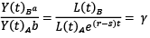
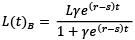
The separate labor units employed in sectors A and B at time t are indicated as L(t)_A and L(t)_b. Similarly, r and s measure the growth of labor productivity in the long run in sectors A and B, respectively. Importantly, the productivity of labor in sector A is presumed to outgrow the productivity of labor in sector B – the Baumol’s sector. Differently from the Baumol (1967) model, this paper assumes that the growth of labor productivity in the Baumol sector is positive. This underlying assumption aligns with the Baumol (1993) notion that service sectors such as health and education are characterized by a slow growth in their productivity, in the long run. Moreover, the parameters a and b are assumed to remain constant. These parameters – a and b – can be regarded as the existing state of technology in the two sectors, respectively. Therefore, taking the ratio of Y_B and Y_A yields bL_B/aL_A e^(r–s)t. Let us assume that the Baumol model attains an equilibrium, thus, the ratio of Y_B andY_A is similar to the proportion of real demand. In both sectors, it decreases over time if real demand is elastic, and the stagnant sector has the likelihood to disappear. However, if the government offers a subsidy to sector B or it becomes inelastic, the ratio between the two sectors can be held constant. Therefore, this proposition can be written as

(3)

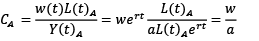
where γ is a constant. In addition, Baumol (1967) assumes that the wage rate per unit of labor employed, w, increases in the two sectors in proportion to the productivity growth of the advancing sector A, r. Furthermore, the rewards for labor in the two sectors are expected to coincide. Thus, the unit cost of labor for the two sectors can be given as

(4)

(5)

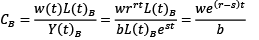
where C_A denotes the unit costs of the advancing sector and is assumed to remain unchanged over time, and C_B represents the unit costs of the stagnant sector which rises continuously following the variance in productivity growth between the two sectors. The latter term is described as the Baumol effect. The wider the interval between r and the growth in productivity in the stagnant sector s, the more extreme the sector is shrunk by the Baumol effect. In line with Hartwig (2008b), it is the same as implying that the unit cost of labor in the stagnant sector rises corresponding to the rise in wage rate above the growth in productivity of the entire economy – the Baumol variable. However, the last-mentioned is concerned with a specific case which is given as follows.

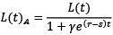
By carrying forward Equation (3), t represents the sum of labor input of the economy at a given time, and L(t) measures the total unit of labor employed in sectors A and B, it can be derived that

(6)

Equation (6) is derived after solving (1)–(3) for L(t)_A and L(t)_B, where L(t) = L(t)_A + L(t)_B. Thus,

(7)

Solving Equations (6) and (7) for L(t)_A and L(t)_B in (1) and (2) yields the following results for total output in the economy:

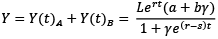(8)

Moreover, dividing Equation (8) by L gives the overall level of labor productivity for the economy.

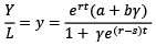(9)

Therefore, the growth of productivity of the entire economy can be given as

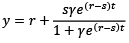(10)

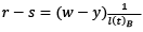
Assuming that r measures the growth rate of wages and taking Equation (7) into consideration, the difference between the surpluses of rise in wages w over and above the growth rate in labor productivity y is

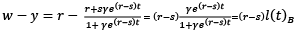(11)

where l_B ≔ L_B/L, and it can be deduced from Equation (11) that the surplus of the growth in wage rate over and above the growth rate in productivity cannot be the same with the growth rate of the stagnant sector, (r – s), until the overall share of the labor supply in the stagnant sector l(t)_B tends to unity. Therefore, (w – y) is what Hartwig (2008b) called the Baumol variable, and indicates that all the labor as a factor of production is engaged in the Baumol sector. Thus, it asymptotically approaches the growth in unit costs of the Baumol sector.

(12)

It is assumed that the growth of productivity for the entire economy asymptotically approaches the growth of productivity for the Baumol sector, s. To date, there is no consensus in the literature regarding the time it will take for the equilibrium of the Baumol model to be attained. Available evidence shows that in developed economies, the share of labor engaged in the progressive sectors has been decreasing, which implies that the largest proportion of the labor is engaged in the stagnant sector of the economy (Schettkat & Yocarini, 2006 ; Colombier, 2017). Consequently, since the average proportion of the overall service sector of the economy is largely less than a hundred percent, testing the Baumol model requires taking the proportion of the labor force in the Baumol sector into full cognizance. Thus, this is performed by adjusting the Baumol variable as the inverse of the proportion of the Baumol sector in the overall workforce.

(13)

Furthermore, to arrive at a compatible result of the dynamics of Baumol’s effect on healthcare expenditure, the right-hand component of Equation (13) has to be emphasized – that is the Baumol variable. Moreover, the remaining component of the same equation is termed as the rate of growth of the unit cost of the Baumol sector.

(14)

Variables and data

The methodology section follows the extant literature by choosing the key drivers of healthcare expenditure, which include per capita income (Hartwig & Sturm, 2018), per capita health expenditures (Bala et al., 2022; Jakovljevic, Sugahara, et al., 2020), elderly population (Jakovljevic, Timofeyev, et al., 2020), physician density (Spinks & Hollingsworth, 2009), and hospital beds (Hitiris, 1997). In addition, life expectancy at birth, mortality rate, and infant mortality are included following the studies of Dreger & Reimers (2005) and (Colombier, 2017). Furthermore, services and the adjusted Baumol variable are included in this study following the work (Colombier, 2017). This paper adds both male and female variables for life expectancy at birth and infant mortality to examine if there is a significant difference between genders and the total population. For the sake of the analysis, all the variables are transformed into logarithmic form. All else constant, advances in medical technology are expected to improve life expectancy at birth and lower mortality from all causes in the entire population. The data used is taken from the World Bank Development Indicators (WDI) for the period of 2000 to 2019. The study countries include Denmark, Estonia, Finland, Germany, Iceland, Latvia, Lithuania, Poland, Norway, Russia, and Sweden. These studied countries are chosen because they have the lowest health outcomes measured in life expectancy at birth and infant mortality relative to the Euro Area, and the OECD countries. Table 1 presents the variables employed in this study and their definitions.

Table 2 reports the trend in health expenditures for the time frame of this study. The PC Crn Hexp increased the most by 606.3% in Sweden, followed by 333.3% in Poland, and 130.4% in Denmark. Similarly, PC Pub Hexp increased by 2028.2% in Latvia, followed by 1794.5% in Lithuania, and 1633.7% in Poland. PC Pvt Hexp increased tremendously by 1593.5% in Denmark, followed by 602.4% in Poland, and 334.5% in Latvia, respectively.

Table 1. Description of the variables

Source: Prepared by the author using WDI data

Table 2. Growth in health expenditures in 1990–2020

Source: Prepared by the author using WDI data

Results

This study used panel data for the 11 countries of Northern Europe and the Baltic region for the period of 2000–2019. The PC Crn Hexp, PC Pub Hexp, and PC Pvt Hexp are used as the dependent variables in the regressions. This is because, on one hand, Baumol views healthcare spending as noninvestment spending (Baumol, 1967). On the other hand, investment expenditure may constitute only a small fraction of healthcare expenditure, not the overall healthcare spending. This has the advantage of examining the effect of both components of healthcare spending on the Baumol model. Moreover, the Baumol model considers the macroeconomic dynamics of healthcare expenditure to circumscribe the aggregate demand effect from Baumol’s effect. Importantly, the aggregate demand effect of healthcare spending is considered the most crucial determinant of healthcare expenditure (Smith et al., 2009). Table 3 presents the panel unit root test where four different tests are performed. It is found that the variables are a combination of stationary and differenced stationary series. Specifically, PC Crn Hexp, PC Pub Hexp, PC Pvt Hexp, PC GDP, death per 1,000 population, physician density, life expectancy, elderly population, infant mortality, and services are all differenced stationary series. However, hospital beds, infant mortality and adjusted Baumol variables are stationary variables.

Table 3. Panel unit root test of the variables

Source: Author’s computation using WDI data. PC Crn Hexp indicates per capita current health expenditure, PC Pub Hexp indicates per capita public health expenditure, PC Pvt Hexp indicates per capita private health expenditure, PC GDP indicates per capita gross domestic product, Services Indicates the total share of service sector measured in value-added as a percentage of gross domestic product, Adj. Baumol. Var. indicates the adjusted Baumol Variable calculated as = (compensation per employee – employment ratio)*1/share of the service sector, *** indicates the significance of the variable at a 1 percent level of significance.

The estimates of the result where PC Crn Hexp is used as the explanatory variable are shown in Table 4. Three estimation techniques – Pooled OLS, Fixed Effects (FE), and Random Effects (RE) – are applied to estimate the model. In model I, though estimates of the three regressions have shown different results, the Hausman test shows a Chi-square value of 10.94 with corresponding p-values of 0.1413 that are statistically insignificant. This suggests that RE regression is the preferred model. Accordingly, the coefficients of the prepared model have explanatory variables which are all significant with signs that are consistent with theoretical expectations. Furthermore, the robustness of model I is ascertained by adding other potential drivers of healthcare expenditures leading to the development of model II for the three types of health expenditures under investigation. These variables include per capita income, life expectancy at birth (male) and (female), and infant mortality (male) and (female). Importantly, adding these variables confirms the estimates of model I that health expenditure exhibit Baumol cost disease, to a different extent, in Northern Europe and the Baltic region. The Hausman specification test is performed to choose the consistent and efficient model between the FE and the RE regressions. Thus, the Hausman test yields a Chi-square value of 20.90 with p-values of 0.0344 that are statistically insignificant. This suggests that estimates of the RE model is efficient, consistent, and prepared in estimating the PC Crn Hexp regression. Similarly, though the Pooled OLS the RE regressions are the same for model II, the results show that PC GDP, death rate per 1,000 people, physician density, and infant mortality (male), are significant and leads to an increase in PC Crn Hexp. However, services are negatively associated with the growth in PC Crn Hexp. Conversely, the FE estimates show that hospital beds, life expectancy at birth (male), infant mortality (total), and the adjusted Baumol variable are not significant. However, the other regressors are significant with signs that are theoretically consistent except the signs of elderly population. Therefore, across the three estimation methods, the adjusted Baumol variable shows a significant coefficient and ranges between 0.01 and 0.05. This suggests that Baumol’s cost disease is significantly associated with PC Crn Hexp in the countries of Northern Europe and Baltic region.

Table 4. Estimates of the current health expenditure regression

Source: Author’s computation using WDI data.

Notes: standard errors are given in parenthesis, *** Significant at 1%, 5% and 10% level, respectively.

Table 5. Estimates of the public health expenditure regression

Source: Author’s computation using WDI data

Notes: standard errors are given in parenthesis, *** Significant at 1%, 5% and 10% level, respectively.

Table 5 shows the estimates of the result where PC Pub Hexp is used as the explanatory variable in the regression. In model 1, though the estimates of the three regressions are different, the Hausman test indicates a Chi-square value of 36.11 with p-values of 0.0000 which is significant. This suggests that the FE model is the prepared model. Thus, in the prepared model, except the coefficient of hospital beds, the coefficients of all the independent variables are significant. However, except the coefficient of infant mortality, the signs of the coefficients are as expected. In addition, although the estimates are the same for Pooled OLS and the RE regression, they differ in the FE regression. In the same way, the Hausman test is applied to choose the prepared model, and it yields a Chi-square value of 108.42 with a p-value of 0.000 that is significant. Consequently, the FE estimates are prepared over the RE regression for analyzing the dynamics of PC Pub Hexp in the countries studied. Furthermore, the three alternative estimates show results that are significant and in favor the adjusted Baumol variable for PC Pub Hexp. It ranges from 0.07 to 5.48 across the three estimation techniques.

Table 6. Estimates of the private health expenditure regression

Source: Author’s computation using WDI data

Notes: standard errors are given in parenthesis *** Significant at 1%, 5% and 10% level, respectively.

In Table 6, the estimates of the result where PC Pvt Hexp is used as the explanatory variable in the regression are presented. In model I, the three estimation techniques present entirely different results and the Hausman test suggests a Chi-square value of 777.59 with corresponding p-values of 0.0000 which is significant. This indicates that the FE results are more efficient and consistent. Therefore, the coefficient of crude deaths, hospital beds, and physician density are both significant and show signs that are consistent with theoretical expectations. Similarly, in model II, the estimates of the Pooled OLS are the same as the estimates of RE regression. Equally, the Hausman test for choosing between FE and RE regressions is applied. It suggests a Chi-square value of 1657.27 with a p-value of 0.000 which is significant, indicating that FE model is more consistent and efficient for analyzing the dynamics of PC Pvt Hexp. Evidence shows that PC GDP, crude deaths, physician density, life expectancy at birth (total), life expectancy at birth, infant mortality (male), infant mortality (female) and the adjusted Baumol variable are both significant and bearing the correct signs. However, infant mortality (total), and services are significant but are bearing alternating signs that are theoretically inconsistent. Therefore, PC Pvt Hexp is significantly associated with the Baumol cost disease in the countries studied.

Discussion

This paper empirically tests the hypothesis that numerous attempts to curb the perennial growth in healthcare expenditures remained pointless since healthcare expenditure epitomizes the Baumol cost disease. Three types of health expenditures – PC Crn Hexp, PC Pub Hexp, and PC Pvt Hexp – are employed in testing the Baumol hypothesis using data for the countries of Northern Europe and the Baltic region from 2000 to 2019. In model 1, death per 1,000 population, physician density, hospital beds, and life expectancy at birth (total), elderly population, infant mortality (total), and services, are used as the drivers for the growth of healthcare expenditures. In addition, the robustness of model I is ascertained by adding other important drivers of healthcare expenditures leading to the estimation of model II for the PC Crn Hexp, PC Pub Hexp, and PC Pvt Hexp, respectively. These variables include per capita income, life expectancy at birth (male) and (female), and infant mortality (male) and (female). Importantly, adding these variables confirms the estimates of (model I) that PC Crn Hexp, PC Pub Hexp, and PC Pvt Hexp partly exhibit the Baumol cost disease, to a different extent, in the countries studied. Specifically, the adjusted Baumol variable for PC Crn Hexp has a coefficient that is statistically significant and ranges in 0.01–0.05 in the two models, and across the three estimations. Therefore, this implies that a one percent rise in the growth rate of the economy in excess of real wages over and above productivity growth adjusted by the inverse of the proportion of overall services in the employment sector will bring about 0.01–0.05 percent rise in the perennial rate of growth in the PC Crn Hexp. Similarly, the adjusted Baumol variable for PC Pub Hexp is significant across the estimation techniques and for both models. It ranges in 0.07–5.48 in the two models suggesting that a rise in the growth rate of the economy will lead to 0.07–5.48 rise in PC Pub Hexp annually, all else is held constant. Moreover, the coefficient of the adjusted Baumol variable for PC Pvt Hexp is significant and ranges in 3.14–6.23 in the two models. This suggests that a one percent rise in the growth rate of an economy in excess of real wages over and above productivity growth adjusted by the inverse of the proportion of overall services in the employment sector will induce rises, valued in 3.14–6.23, in the perennial rate of growth of PC Pvt Hexp. Findings similar to this are reported in prior studies conducted by Atanda et al. (2018), Wang & Chen (2021), Hartwig (2008a), (Colombier, 2017), and (Bates & Santerre, 2013). The result conflicts with Hartwig’s studies (Hartwig, 2008a), (Hartwig & Sturm, 2018).

Moreover, as a crucial driver of healthcare spending, the coefficient of PC GDP introduced in model II is highly significant across the alternative estimation techniques. In addition, its income elasticity is below unity for the three types of health expenditure under investigation.. Therefore, this suggests that current health expenditure, public and private health expenditure are seen as a luxury in this context. Regarding the coefficient of income elasticity, this finding is consistent with the findings of published studies which include the works (Colombier, 2017), (Hartwig & Sturm, 2014), (Martín et al., 2011), (Colombier, 2012) and (Costa-Font et al., 2011). The coefficient for the elderly population is significant only in three estimations for PC Crn Hexp. However, bearing the theoretical expectation sign, the coefficient of the elderly population is not at all significant in the four estimations for PC Pub Hexp. The coefficient of physician density turns out to be positive and significant in all the estimations for PC Crn Hexp, PC Pub Hexp, and PC Pvt Hexp. Furthermore, the traditional proxies for health outcomes included as the determinants of health expenditures – life expectancy at birth (total) and infant mortality (total) – show mixed results for PC Crn Hexp. Thus, life expectancy at birth (total) turns out to be significant in four regressions, and the signs are as expected. Infant mortality (total) is significant and bears the correct sign in the three different estimations (model I), and it’s significant with alternate sign in only one regression (model II). In the same way, life expectancy at birth (total) is significant with correct signs in the six regressions for PC Pub Hexp. Infant mortality (total) is significant with an alternate signs in two regressions (model I). Additionally, life expectancy at birth (total) is significant with correct sign in four regressions for PC Pvt Hexp. The same is true for infant mortality (total) in four regressions. Noteworthy, the F-tests suggest that the estimates are robust and significant across the alternative estimation techniques. This evidence is in line with the results of (Smith et al., 2009), Colombier (2017), and Colombier (2012). Therefore, to policymakers, these results suggest that there are many possibilities to be explored to suppress the perennial growth in healthcare expenditures relative to the available avenues debated in the contemporary literature of health economics. In addition, part of the findings of this study that the secular rise in PC Pvt Hexp may not be connected with Baumol’s cost disease may warrant future investigation. However, for the three types of health expenditures analyzed, findings support the Baumol cost disease hypothesis, they seem to suggest that the surge in health care expenditure cannot be overcome using the traditional approach that many have talked about in the literature. These findings suggest that achieving a balance growth in different sectors of the studied countries may result in disentangling the health sector from the Baumol’s effects. Moreover, it is evident that private health expenditure has a comparatively larger effects than those observed in current and public health expenditure. The theoretical and practical implications of these findings seem to suggest that labor growth in the health sector of the studied countries consume more of private health services. Improvement in technology related to health may lead to higher substitutability of capital for labor in the health sector. Consequently, there is a need for a progressive technological improvement that could cut health care expenditure and provide better population’s health outcomes.

Conclusion

This study tests the Baumol hypothesis using panel data for the countries of Northern Europe and the Baltic Region in the period of 2000–2019. The analysis used the adjusted Baumol variable derived from the already developed in the literature and tested Baumol hypothesis using three different types of healthcare expenditures. The results highlight that there is sufficient evidence, partly, in favor of the Baumol cost disease hypothesis for the three types of health expenditures analyzed. Consequently, in the two models, current health expenditure may have grown from 0.01 to 0.05 due to the effects of Baumol’s cost disease. Similarly, public health expenditure may have increased from 0.07 to 5.48 due to the effect of Baumol’s sector. Lastly, private health expenditure may have increased from 3.14 to 6.23 due to the same effect of the Baumol’s sector. Therefore, if the economy is to maintain a steady growth in its different sectors, the Baumol’s effect is likely to disappear in the health sector of the countries studied. However, this study is not without limitations. The growing change in the dynamic of diseases and technological progress across the World will lead to a continuous rise in health expenditures. This study only tested the Baumol’s effect without fully taking into account of the technological and disease dynamics of the population. If data will be available, future studies will examine the impact of technology and disease specific effects on the growth of health expenditure.

References

Atanda, A., Menclova, A. K., & Reed, W. R. (2018). Is health care infected by B aumol’s cost disease? Test of a new model. Health Economics, 27(5), 832–849.

Bala, M. M., Singh, S., Kumar, N., & Janor, H. (2022). Predicting key drivers for health care expenditure growth in the Middle East region: A Grossman-PLS modeling approach. Expert Review of Pharmacoeconomics & Outcomes Research, 22(6), 1021–1031.

Baltagi, B. H., & Moscone, F. (2010). Health care expenditure and income in the OECD reconsidered: Evidence from panel data. Economic Modelling, 27(4), 804–811.

Barkat, K., Sbia, R., & Maouchi, Y. (2019). Empirical evidence on the long and short run determinants of health expenditure in the Arab world. The Quarterly Review of Economics and Finance, 73, 78–87.

Bates, L. J., & Santerre, R. E. (2013). Does the US health care sector suffer from Baumol’s cost disease? Evidence from the 50 states. Journal of Health Economics, 32(2), 386–391.

Baumol, W. J. (1967). Macroeconomics of unbalanced growth: The anatomy of urban crisis. The American Economic Review, 57(3), 415–426.

Baumol, W. J. (1993). Health care, education and the cost disease: A looming crisis for public choice. In The next twenty-five years of public choice (pp. 17–28). Springer.

Colombier, C. (2012). Drivers of health care expenditure: Does Baumol’s cost disease loom large?

Colombier, C. (2017). Drivers of Health‐Care Expenditure: What Role Does Baumol’s Cost Disease Play? Social Science Quarterly, 98(5), 1603–1621.

Costa-Font, J., Gemmill, M., & Rubert, G. (2011). Biases in the healthcare luxury good hypothesis?: A meta-regression analysis. Journal of the Royal Statistical Society Series A: Statistics in Society, 174(1), 95–107.

Dreger, C., & Reimers, H.-E. (2005). Health care expenditures in OECD countries: A panel unit root and cointegration analysis.

Elmi, Z. M., & Sadeghi, S. (2012). Health care expenditures and economic growth in developing countries: Panel co-integration and causality. Middle-East Journal of Scientific Research, 12(1), 88–91.

Hartwig, J. (2008a). Has Health Capital Formation Cured’Baumol’s Disease’? Panel Granger Causality Evidence for OECD Countries.

Hartwig, J. (2008b). What drives health care expenditure?—Baumol’s model of ‘unbalanced growth’revisited. Journal of Health Economics, 27(3), 603–623.

Hartwig, J., & Sturm, J.-E. (2014). Robust determinants of health care expenditure growth. Applied Economics, 46(36), 4455–4474.

Hartwig, J., & Sturm, J.-E. (2018). Testing the Grossman model of medical spending determinants with macroeconomic panel data. The European Journal of Health Economics, 19(8), 1067–1086.

Hitiris, T. (1997). Health care expenditure and integration in the countries of the European Union. Applied Economics, 29(1), 1–6.

Jakovljevic, M., Sugahara, T., Timofeyev, Y., & Rancic, N. (2020). Predictors of (in) efficiencies of healthcare expenditure among the leading asian economies–comparison of OECD and non-OECD nations. Risk Management and Healthcare Policy, 2261–2280.

Jakovljevic, M., Timofeyev, Y., Ranabhat, C. L., Fernandes, P. O., Teixeira, J. P., Rancic, N., & Reshetnikov, V. (2020). Real GDP growth rates and healthcare spending–comparison between the G7 and the EM7 countries. Globalization and Health, 16(1), 1–13.

Ke, X. U., Saksena, P., & Holly, A. (2011). The determinants of health expenditure: A country-level panel data analysis. Geneva: World Health Organization, 26(1–28). https://r4d.org/wp-content/uploads/TransisitionsInHealthFinancing_DeterminantsofExpenditures.pdf

Martín, J. J. M., Puerto Lopez del Amo Gonzalez, M., & Dolores Cano Garcia, M. (2011). Review of the literature on the determinants of healthcare expenditure. Applied Economics, 43(1), 19–46.

Murthy, V. N., & Okunade, A. A. (2016). Determinants of US health expenditure: Evidence from autoregressive distributed lag (ARDL) approach to cointegration. Economic Modelling, 59, 67–73.

Nordhaus, W. D. (2008). Baumol’s Diseases: A Macroeconomic Perspective. The B.E. Journal of Macroeconomics, 8(1). https://doi.org/10.2202/1935-1690.1382

Schettkat, R., & Yocarini, L. (2006). The shift to services employment: A review of the literature. Structural Change and Economic Dynamics, 17(2), 127–147.

Smith, S., Newhouse, J. P., & Freeland, M. S. (2009). Income, insurance, and technology: Why does health spending outpace economic growth? Health Affairs, 28(5), 1276–1284.

Spinks, J., & Hollingsworth, B. (2009). Cross-country comparisons of technical efficiency of health production: A demonstration of pitfalls. Applied Economics, 41(4), 417–427.

Triplett, J. E., & Bosworth, B. (2003). Productivity measurement issues in services industries: Baumol’s disease has been cured. Economic Policy Review, 9(3). https://papers.ssrn.com/sol3/papers.cfm?abstract_id=789545

Wang, L., & Chen, Y. (2021). Determinants of China’s health expenditure growth: Based on Baumol’s cost disease theory. International Journal for Equity in Health, 20(1), 1–11.

World Bank. (2012). World development indicators 2012. The World Bank.

Werblow, A., Felder, S., & Zweifel, P. (2007). Population ageing and health care expenditure: A school of ‘red herrings’? Health Economics, 16(10), 1109–1126. https://doi.org/10.1002/hec.1213

Yetim, B., İlgün, G., Çilhoroz, Y., Demirci, Ş., & Konca, M. (2021). The socioeconomic determinants of health expenditure in OECD: An examination on panel data. International Journal of Healthcare Management, 14(4), 1265–1269. https://doi.org/10.1080/20479700.2020.1756112

Zweifel, P., Felder, S., & Meiers, M. (1999). Ageing of population and health care expenditure: A red herring? Health Economics, 8(6), 485–496. https://doi.org/10.1002/(SICI)1099-1050(199909)8:6<485::AID-HEC461>3.0.CO;2-4