Ekonomika ISSN 1392-1258 eISSN 2424-6166

2025, vol. 104(1), pp. 6–29 DOI: https://doi.org/10.15388/Ekon.2025.104.1.1

Decline of Interest Rates under Inflation Targeting and Previous Regimes: Evidence from Latin America and Developed Countries

Sergio Julio Chión-Chacón
CENTRUM Católica Graduate Business School, Lima, Perú
Pontificia Universidad Católica del Perú, Lima, Perú
Email: sjchion@pucp.edu.pe
ORCID: https://orcid.org/0000-0002-7955-3163

Kevin Antonio Álvarez García
CENTRUM Católica Graduate Business School, Lima, Perú
Pontificia Universidad Católica del Perú, Lima, Perú
Email: kevinz.kag@gmail.com
ORCID: https://orcid.org/0000-0003-0037-4865

Abstract. This study empirically investigates the impact of Inflation Targeting (IT) on nominal interest rates over the past 40 years, focusing on 10 advanced and emerging economies. By using a Binary Regime Model embedded within a Backward-Looking Taylor, our findings confirm that IT adoption has significantly contributed to reducing interest rates, with the strongest effects observed in Latin American countries. To reinforce these results, we incorporate Smooth Transition Regression (STR) models, with and without instrumental variables, allowing for a more suitable representation of gradual policy transitions. The STR estimates consistently support our main findings, validating the robustness of the observed impacts. Furthermore, we show that, both before and after IT implementation, central banks display a stronger emphasis on responding to inflation than to the output gap, with this focus intensifying under IT regimes.
Keywords: Monetary policy, inflation targeting, interest rates, Taylor Rule, Smooth Transition Regression.

___________

Received: 15/09/2024. Revised: 20/12/2024. Accepted: 05/01/2025
Copyright © 2025 Sergio Julio Chión-Chacón, Kevin Antonio Álvarez García. Published by Vilnius University Press
This is an Open Access article distributed under the terms of the Creative Commons Attribution License, which permits unrestricted use, distribution, and reproduction in any medium, provided the original author and source are credited.

1. Introduction

In the last 40 years, interest rates have exhibited a clear decreasing trend in both developed and emerging economies¹ (Li, 2012; Bernanke, 2022). Despite the global economy going through various expansionary and contractionary phases, even with significant fluctuations in short-term interest rates, the long-term trend remains intact. Many arguments have been put forth regarding the factors behind this reduction.

Bernanke (2022) emphasizes that the decline in inflation could have been a decisive factor, as lenders tend to demand lower premiums (interest rates) when inflation is reduced. This observation underscores the importance of understanding the mechanisms that have led to a decrease in inflation as a relevant contributing factor. Moreover, the literature shows that the determinants of interest rates have an important relationship with the monetary policy framework (Bambe, 2023).

Empirical studies have shown that inflation targeting regimes have been successful in maintaining low, stable, and less volatile inflation levels (Mishkin and Schmidt-Hebbel, 2007; Vega and Winkelried, 2005; Visokaviciene, 2010; Stojanovikj and Petrevski, 2020; Arsić et al., 2022; Bhalla et al., 2023). Therefore, while there is substantial literature on the effectiveness of inflation targeting in stabilizing inflation, there are no studies that directly explore its impact on nominal interest rates. Our study seeks to fill this gap by examining the role of inflation targeting in reducing interest rates, focusing on the pre- and post-IT periods in both emerging and advanced economies. This comparative analysis of the periods before and after the adoption of IT is a key innovation of our research, offering new insights into the mechanisms behind interest rate dynamics.

The transmission mechanism is quite intuitive. If inflation targeting (IT) generates a climate of trust and credibility, it will anchor inflation expectations and result in lower long-term inflation, thereby leading to a reduction in interest rates. Additionally, the adoption of IT may encourage a greater fiscal discipline (Apeti et al., 2024), which could, in turn, contribute to lowering both inflation and interest rates.

Understanding whether IT has been an important factor in the falling rates becomes fundamentally important because it would demonstrate the effectiveness of inflation targeting as a monetary policy tool to promote not only price stability but also more favorable financial conditions. Practically, this could support the credibility and confidence in the monetary policies implemented by the central banks that adopt these targets.

Figure 1. Interbank interest rate and Treasury Yields

Note: Figure 1 (a) shows the average of the interbank interest rate in IT the regime and before. The total sample covers from 1962Q2 to 2022Q4 (the start date varies among countries), whereas the periods in IT start from 1992 to 2022 (see Table 1). For Brazil, periods with atypical interest rates are omitted, and the sample from 1995Q3–1999Q2 is considered as pre-IT. The rate for Japan is 0.36 before IT and 0.07 in IT; for graphical purposes, we multiply these values by 10. Source: Federal Reserve Economic Data (FRED).

The objective of this study is to explore whether Inflation Targeting (IT) has played a role in the historical decline of interest rates observed across a sample of representative economies from both emerging and advanced countries. Also, we study if inflation and the output gap play any role in the process of pursuing the inflation target by central banks. To address this issue, we estimate a binary switching regression embedded within a backward-looking Taylor Rule while using the ordinary least squares (OLS) regression model.

Table 1. Inflation Targeting Adoption

Note: The length of the inflation target varies among nations. In the cases of Peru and the United Kingdom, the target is established indefinitely, encompassing all periods. Chile’s inflation target spans approximately two years. Meanwhile, Colombia and Mexico employ a medium-term target, while Brazil opts for a yearly target. Lastly, Canada’s inflation target extends over a period of six to eight quarters. The inflation targets of 2022 are considered as current targets. Sources: Bank of England and Reuters.

The use of a backward-looking Taylor Rule is justified by several considerations. First, forward-looking rules rely on expectations of inflation and output gaps, which are often subject to measurement errors and unreliable real-time data (Mankiew et al., 2004; Reid and Siklos, 2021). Backward-looking rules, by focusing on observed historical data, minimize these issues and reduce the potential endogeneity concerns. Additionally, such rules help ensure determinacy in structural models, as highlighted in the literature (Carlstrom and Fuerst, 2000), where backward-looking rules contribute to stable and unique equilibria. While an extension of this analysis could involve the consideration of a forward-looking rule, the backward-looking approach remains robust for the purposes of this study and aligns with empirical evidence in historical contexts.

We utilize a simple regression model estimated under OLS since there is recent evidence that this estimation method performs better in estimating Taylor-type rules (Carvalho et al., 2021). The analysis is conducted for a set composed of Advanced economies and of Latin American economies (US, UK, Canada, Japan, Euro Area, Peru, Chile, Colombia, Mexico, and Brazil) that have adopted Inflation Targeting (see Table 1). Additionally, to analyze and compare the variations of the rates in both periods, elasticities are calculated in both regimes.

Our article contributes to the literature by expanding empirical evidence on the effect of Inflation Targeting (IT) in reducing the interest rates, particularly in emerging Latin American economies. It further contrasts these experiences with those observed in the developed countries, thus providing a comparative analysis which is bound to highlight differences and similarities in the impact of IT across varying economic contexts.

The empirical results show that the adoption of IT has played a substantial role in lowering the interest rates in recent years, particularly with a stronger impact being observed in Latin American economies. Also, our analysis reveals that central banks have exhibited a more pronounced response to inflation compared to the output gap, both prior to and following the implementation of inflation targeting (IT), and the response of central banks to inflation has shown an upward trend after the adoption of IT.

The following sections proceed as follows. Section 2 provides a brief literature review. Section 3 demonstrates the methodology applied in this study. Section 4 presents the obtained results and discusses the relevant considerations and facts. Finally, in Section 5, conclusions are presented.

2. Literature Review

The relationship between inflation targeting (IT) and interest rates has been the subject of extensive research, yet the evidence remains mixed. For instance, Fouejieu and Roger (2013) explore how IT influences cross-country interest rate spreads in both emerging and advanced economies. By using a dynamic panel data approach and system GMM to address endogeneity, they find that IT leads to a decline in country risk premium spreads, particularly under conditions of a reduced political uncertainty.

Similarly, De Mendoça and Souza (2009) examine the relationship between the monetary policy credibility and interest rates. By constructing a novel credibility index based on expert surveys, they demonstrate through OLS regression that, during the IT period, interest rates exhibited less variability due to an enhanced monetary policy credibility.

Alternatively, Gehringer and Mayer (2019) investigate the factors driving nominal long-term interest rates. By using a VAR model with a DOLS procedure, they conclude that, in major industrialized economies, central banks’ monetary policies have significantly contributed to maintaining low interest rates. They argue that the close connection between short-term rates (controlled by central banks) and long-term rates is more reflective of central bank perceptions than those of the market participants.

The studies supporting a positive effect of IT on interest rates generally argue that IT fosters a climate of confidence and expectation management, leading to consistent reductions in interest rates. Additionally, other research highlights a strong link between the inflation control and lower interest rates. For example, Fazlollahi and Ebrahimijan (2022) provide econometric evidence of a bidirectional causality between interest rates and inflation rates in Canada, thereby supporting Bernanke’s (2022) premise that inflation rates significantly influence historical interest rates.

However, not all research supports the hypothesis that IT has a substantial impact on interest rates. Lin and Ye (2007), by using Propensity Score Matching, find that IT does not significantly affect inflation or inflation variability in industrialized countries. Similarly, Ball and Sheridan (2005), by employing a difference-in-differences model, find that IT does not exert significant effects on long-term interest rates in advanced economies. They attribute the observed inflation decline to a mean-reversion phenomenon rather than to IT itself.

Beyond IT, other factors have been identified as influencing the decline in real interest rates. For instance, research by Dell’Erba and Sola (2016), Barnejee et al. (2022) and Kregzde and Murauskas (2015) points to a strong relationship between fiscal policy management and interest rates. The above-listed authors argue that reducing spreads can lower other interest rates in the economy. However, Dautovic (2017) claims that the relationship between fiscal policy variables – such as government spending or budget deficits – and long-term interest rates tends to weaken or even disappear once the persistent nature of interest rates has been accounted for in econometric models. Another crucial factor is the ‘global saving glut’, a concept introduced by Bernanke (2005a), which refers to a worldwide increase in savings, leading to reduced interest rates. Bernanke identifies demographic changes and income growth as the key drivers of this global savings increase. While supporting this view, Barsky and Easton (2021) argue that the global saving glut hypothesis explains the decline in long-term real interest rates from 2002 to 2006 but may not fully account for the further decrease observed after the Great Recession.

Upon reviewing the literature, several considerations emerge. First, studies relying on expectation data may be flawed. In this context, Reid and Siklos (2021) highlight that measuring inflation expectations is challenging due to their unobservable nature and the respondents’ misunderstanding of economic concepts, leading to biased and inconsistent data. Second, much of the empirical literature focuses on advanced industrialized countries, thereby limiting the generalizability of the findings. These countries had a low inflation and more efficient institutions even before adopting IT. Finally, studies using treatment effects may be biased. For example, difference-in-differences models that do not account for time-varying treatment effects can introduce bias (Goodman-Bacon, 2021). Moreover, if countries in the sample are not genuine inflation targeters but behave as such, the estimated treatment effects may be misleading.

This research seeks to fill these gaps by providing evidence for emerging Latin American countries. Instead of relying on expectation data, we adopt a more straightforward and methodologically robust approach to address these issues.

3. Method

3.1. Research Model

3.1.1. Binary Regime Model

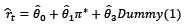
We estimate regressions of the Backward-Looking type Taylor Rule for ten different countries as follows:

(1)

where r_t is the nominal interbank interest rate, π is the inflation rate gap, while is the output gap (defined as the percentage difference between the output and its long-term trend level). Central to our analysis is the introduction of a dummy variable, D_t, which takes the value of ‘1’ during the inflation targeting period and ‘0’ otherwise. This allows us to capture the effects of both the inflation targeting period and the preceding monetary policy regimes.

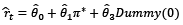
We use the Ordinary Least Squared (OLS) method to estimate the coefficient of the regressions for both Latin American and developed countries. We capture the estimator for the two monetary policy regimes as follows:

; I.T. regime

; previous regimes

Endogeneity in structural models like the Taylor Rule can lead to biased estimators. The common approach in the literature is to use Instrumental Variables (IV) or GMM (Maher et al., 2022; Horvath et al., 2022). However, ensuring the exogeneity and validity of instruments, especially in time series, is challenging. Empirical evidence suggests that Ordinary Least Squares (OLS) provides a better performance as well as a smaller endogeneity bias in reasonably sized samples (Carvalho et al., 2021). Following Miles and Schreyer (2012) and Carvalho et al. (2021), we opt for OLS instead of 2SLS². To address serial correlation, heteroskedasticity, and autocorrelation, we use HAC standard errors and bootstrap techniques.

3.1.2. Smooth Transition Regression (STR)

The smooth transition model captures gradual changes in the structural parameters of an equation, as opposed to abrupt shifts, thus making it particularly useful for analyzing policies with potential regime changes. In this context, the model incorporates a transition dynamic which depends on a threshold variable (such as the temporal distance from the implementation date of a regime). We estimate the model both without and with instrumental variable (IV) estimation to address potential endogeneity issues. The general form of the model is:

(2)

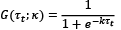
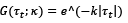
In this model,r_t represents the interbank interest rate, is the inflation rate relative to its target, and is the output gap. G(τ_t; κ) is the transition function, which depends on the threshold variable τ_t (in this case, representing the temporal distance from the date of IT adoption), and κ is the smoothness parameter. In this framework, two types of transition functions are feasible, as follows:

Logistic function

Exponential function:

The selection between the two functions is made by minimizing the sum of squared residuals (SSR) for different values of the smoothness parameter 𝜅³. To address potential inference issues caused by severe autocorrelation, Bootstrap was used to estimate the standard errors of the model⁴. Therefore, under this specification, the aim is to address (i) the gradual nature of the effects of IT adoption, (ii) potential endogeneity issues, and (iii) possible autocorrelation problems by providing a more robust estimation of the standard errors, thereby enhancing the reliability of the results.

3.2. Data and Variables

We collected quarterly data on the interbank interest rate, inflation and output for the ten countries included in our sample. The specific variables employed were dictated by the best data available. We follow Miles and Schreyer (2012), who used a measure of short term interest rates⁵. For the developed economies and Brazil, we use the 3-month interbank rate⁶. For Mexico, we use the ‘28 days interbank rate’, while for Peru, Chile and Colombia, we refer to the 1-day interbank rate. The interbank rate, the inflation, and the real output were taken from the Federal Reserve Economic Data (FRED), Economic Commission for Latin America (CEPAL) the International Monetary Fund (IMF) and the central banks websites of each country to be analyzed. We consider the inflation rate as the year-to-year variation of the Consumer Price Index (CPI). This measure includes the interannual variation of the quarterly average⁷ of CPI 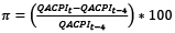. The output gap was obtained by the Hodrick-Prescott filter⁸.

According to the sample, Canada has the largest data series, running from 1962Q1 to 2022Q4. It is followed by the United States, with the data spanning the period from 1964Q3 to 2022Q2. The United Kingdom’s data run from 1986Q1 to 2022Q2. The Euro Area provides data from 1995Q1 to 2022Q4, while Japan’s data run from 2002Q2 to 2022Q4.

For the Latin American economies, Brazil runs data from 1994Q4 to 2022Q4, while Mexico and Colombia can be sourced from 1995Q2 to 2022Q4. Peru’s data run from 1995Q4 to 2022Q4, and, finally, Chile offers data from 1996Q1 to 2022Q4.

Table 2 shows the main patterns followed by both inflation and interest rates. In general, the average inflation levels have fallen for all the countries analyzed that adopted IT with the exception of the Eurozone and Japan. In terms of magnitude, emerging countries have maintained the highest levels of average inflation compared to the developed economies, both before and after the implementation of the inflation targeting (IT) frameworks. Likewise, the volatility levels after the adoption of IT have been reduced for the majority of the countries in the sample (with the exception of the Eurozone and Japan, from 0.32 to 1.7, and 0.76 to 1, respectively), which would indicate that the adopted monetary policy regime or rule has had an impact on maintaining a stable level of inflation. Similarly, it is noteworthy that both inflation and interest rates consistently exhibit medians that are lower than their respective averages in both regimes. This provides insights into the data distribution and suggests a rightward bias that may be influenced by outliers.

Table 2. Summary statistics on inflation and interbank interest rate (% annual rates)

Note: The data in this table are presented in quarterly frequency. The sample prior to inflation targeting was chosen based on the availability of data. The data sample for each country corresponds exactly to the one specified in the data section. Sources: Federal Reserve Database (FRED) and Central Banks of each country.

Correspondingly, interest rates have followed the same pattern as inflation. All countries analyzed have shown both a reduction in average rates and a drop in volatility after the adoption of IT. The emerging countries of Latin America are those that have had a greater reduction in rates compared

to the developed countries. Thus, the data would preliminarily show that the IT regime could have influenced these downward trends in the interest rates and their volatility (Rossetti et al., 2017).

4. Results

The results reported in Table 3 provide empirical evidence that the adoption of IT has played a significant role in reducing the interest rates in both advanced and Latin American economies. The estimated coefficient of dummy variables included in the model (capturing the inflation targeting regime) are negative and statistically significant at a confidence level of 99% for all the countries considered in our sample.

The negative signs are as expected, indicating that the adoption of IT has generated an effect in the reduction of the rates. Based on the magnitudes, the estimated coefficients for the dummy variables represent to what extent the adoption of IT has contributed to the reduction of the interest rates in percentage points. Therefore, it can be observed that the estimated coefficients of the dummy variables for the Latin American economies range from -11.10 to -8.36, which correspond to Brazil and Mexico, respectively. In contrast, for advanced economies, the range varies from -7.56 to -0.34, representing the UK and Japan, respectively. This result implies that the monetary policy strategy under IT has played a more significant role in the emerging economies.

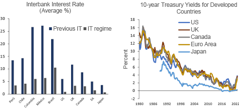
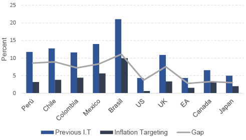
The implication of these results can be appreciated through the model’s estimates of the interbank interest rate at the inflation target level and the output at its potential level, as shown in Figure 2. Figure 2 illustrates the model’s estimates of the interbank interest rate. For this, we base our analysis on the assumption that inflation is at its target level and that the output is at its potential level. Prior to the adoption of inflation targeting (IT), the estimated interest rates for the Latin American countries, except for Brazil, do not exceed 15%. However, following the implementation of IT, the rates for the countries in this group do not exceed 5.6%. The estimates for the developed countries exhibit a similar pattern as, prior to the adoption of inflation targeting (IT), interest rates did not exceed 11%. However, following the implementation of IT, the rates for these countries do not exceed 3.3%. It is of importance to note that the difference in the interest rates between these two periods is captured by the coefficients of the previously estimated dummy variables.

One advantage of the proposed model is that it enables us to understand the behavior of central banks in their role of maintaining inflation at its target level and minimizing the output gap. This allows us to assess whether central banks exhibit a stronger response to inflation or to the output gap, as well as whether they adhere to a backward-looking rule.

To ensure the robustness of our findings, we also estimated the model using instrumental variables IV, as shown in Table 9. However, the IV results were less reliable, with larger standard errors and some counterintuitive coefficient signs. These limitations are likely due to weak instruments, as the lags of inflation and output gaps used as instruments may fail to adequately explain the endogenous variables. Consequently, the baseline model remains the preferred specification.

Table 3 displays the statistical significance of inflation for the Latin American countries, where Peru, Chile, Colombia, and Mexico exhibit significant results. Among these countries, only Peru, Chile, and Colombia maintain statistical significance for the output gap as well. It is evident from the analysis that the central banks of these countries have displayed a stronger response to inflation compared to the output gap within the sample considered. The central bank of Colombia has exhibited the highest response to inflation with a coefficient of 0.89, whereas Chile has shown the highest response to the output gap with a coefficient of 0.35.

On the other hand, within the group of the developed economies, the United States, Canada, and Japan exhibit significance in relation to inflation, whereas only Canada displays significance in terms of the output gap. This finding aligns with the results observed in the emerging economies, as Canada (representing the developed economies) also demonstrates a stronger response to inflation than the output gap. Furthermore, it is noteworthy that the Federal Reserve (Fed) demonstrated the most robust response to inflation among the countries in this group, with a coefficient of 0.75.

Taking a broader perspective, when considering both the advanced and the Latin American economies that displayed statistical significance in either inflation or the output gap, it becomes evident that Colombia exhibited the strongest response to inflation, while Canada demonstrated the most significant response to the output gap.

Therefore, considering estimations with at least one variable with statistical significance between inflation and the output gap, for 7 of the ten countries, central banks adhere to a backward-looking Taylor Rule (Equation (1)). Within these seven countries, the Taylor Rule shows significance for both variables for Peru, Chile, Colombia, and Canada. For the other three countries, estimations show significance for only inflation for Mexico, the United States and Japan. Notably, there is no country with only significance for the output variable, beside the dummy. As mentioned above, Brazil, UK, and the Euro area show no significance with the backward-looking Taylor Rule, but the significance of their dummies, indeed, shows the influence of the targeting rule in their interest rate levels.

The coefficient of determination is examined for those countries which adhere to a backward-looking rule or maintain statistical significance in at least one variable. Upon analysis, it is observed that Latin American countries exhibit a high level of adjustment, with an explanatory range ranging from 0.75 to 0.92. This suggests that both inflation and the output gap were the most influential variables considered by their central banks. However, in the case of Brazil, where significance is not maintained in any variable except for the dummy variable, it indicates that the central bank may have responded to other macroeconomic variables which are not included in our model.

In the case of developed economies, the coefficient of determination values is lower compared to those of Latin American countries, with an adjustment range measuring between 0.44 and 0.68. Regarding Brazil, the United Kingdom, and the Euro Area, it is possible that other variables could account for the behavior of their central banks.

Table 3. O.L.S estimation of Equation (1)

Notes: Standard errors are given in parentheses. The asterisks denote statistical significance at the 1 (***), 5 (**), and 10 (*) percent levels. Standard errors were calculated by the HAC robust estimator.

Moreover, we calculate the elasticities of both the inflation and the output gap for all the countries in our sample. Table 4 presents the inflation and output elasticities (see Appendix A) for countries with statistical significance before and after the adoption of IT, considering the economy operating at its potential level and with inflation in its target level. It is of importance to note that, in both regressions (pre- and post-IT), the slope remains constant within each country. What differs is the interest rate level, that is, the intercept.

Table 4. Inflation and output Elasticity under inflation target and potential GDP

Notes: this section considers the target of inflation as an average weight by the dwell time of the target. The ratio is the division between the IT period and before IT. For output elasticities, we consider the average of the potential output. All the ratios are shown in absolute values.

(3)

(4)

Elasticity of inflation = (5)

Elasticity of output gap = (6)

In general, the inflation elasticities of the emerging economies in Latin America before the IT regime range from 0.07 to 0.14, while, under the inflation targeting regime, the range of elasticities is from 0.27 to 0.37. A similar pattern is observed in the developed economies, with the United States, Canada, and Japan experiencing the greatest relevance of inflation in magnitude. Overall, it is evident that, in the Latin American economies, Colombia and Mexico demonstrate a stronger response to inflation prior to the adoption of IT (see Table 4) However, after the implementation of IT, Chile emerges with the highest response to inflation, by virtue of exhibiting an elasticity of 0.37. Similarly, among the developed economies, the United States shows a greater response to inflation compared to its counterparts prior to and after the introduction of IT. These findings corroborate previous results, indicating that central banks in both advanced and emerging economies have exhibited a more pronounced reaction to inflation than to the output gap. Finally, we can infer two crucial points. Firstly, the central banks in our sample have exhibited a stronger response to inflation compared to the output, both before and after the adoption of information technology (IT). Secondly, following the implementation of IT, the response to inflation has experienced a significant increase.

Figure 2. Interbank rate estimation under inflation targeting and previous regimes

Notes: The estimates in Figure 2 come from regressions (Equations (5) and (6)). The interest rate for Japan before IT is 0.5, and after IT is 0.2. For graphical reasons, we multiply them by 10.

The results presented above rely on the assumption that the implementation of inflation targeting (IT) had immediate effects rather than gradual ones. While these earlier results align well with the data, it is worth evaluating whether the policy change was indeed gradual, as this would allow us to validate our previous findings.

For this purpose, Equation (2) is estimated by using Smooth Transition Regression (STR). Given that the Taylor Rule applied here is backward-looking, endogeneity issues are unlikely to arise. Nevertheless, in order to enhance the robustness of our analysis, we estimate an additional model by using instrumental variables (IV).

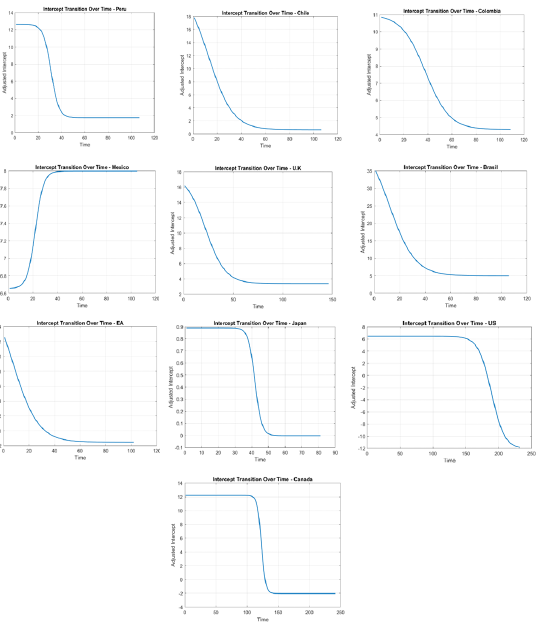
The inflation gap and the output gap variables are treated as endogenous, and their lags are used as instruments. Table 6 presents the baseline model results without considering instrumental variables. The findings indicate that the transition variable, which captures the gradual effect of the policy shift, is statistically significant and negative across all the countries under investigation. This supports the hypothesis that the transition to IT was gradual, and that IT contributed to the reduction of nominal interest rates. The intercepts, which represent the average nominal interest rates in the absence of cyclical fluctuations, show a significant decline following the adoption of IT.

Figure 5 addresses potential endogeneity issues. The results reveal considerable variation in parameter estimates and their standard errors, thus suggesting potential endogeneity in the baseline model. Only in Peru, Chile, the UK, Canada, the Euro Area, and Japan there exists the transition variable, representing the gradual effect of IT adoption, which is statistically significant and negative. Furthermore, some parameter signs appear counterintuitive – for instance, in Japan, the UK, and Canada – although these coefficients are not statistically significant.

Table 5. Smooth transition regression model estimated using instrumental variables (IV)

Notes: The smooth transition regression model used a continuous logistic function in all cases, after evaluation of the nonlinear test based on Teräsvirta (1994). The model uses estimates under instrumental variables (IV), where the instruments were the lags (2) of the independent variables. It is worth noting that the results are subject to the possible weakness of the instruments. The standard error in parentheses was estimated by using the bootstrap method with 2000 iterations.

Table 6. Smooth transition regression model estimated by OLS

Notes: The smooth transition regression model used a continuous logistic function in all cases, after evaluation of the nonlinear test based on Teräsvirta (1994). The standard error in parentheses was estimated by using the bootstrap method with 2000 iterations.

These findings can be summarized as follows: there is evidence suggesting the existence of endogeneity, which implies that the most reliable results are those in Table 5. In countries where a smooth transition is not observed, the earlier results (Table 3) indicate that an abrupt transition explains the data better. This could be due to the fact that, although countries have an official IT implementation date, they may have already maintained an implicit target range before the official announcement⁹. This would mean that the smooth transition occurred prior to the official IT date, while the stronger effects were captured as an abrupt change. Conversely, in countries where smooth transitions are evident, it is likely that they did not adopt preemptive measures akin to an IT regime before its formal implementation. Transitions may vary in magnitude and speed across countries, as shown in Figure 3. In all cases, the evidence supports the premise that IT contributed to reducing the interest rates.

If the IT regime has contributed to the reduction of the nominal interest rates, it likely indicates a stronger anchoring of inflation expectations, leading to more stable and lower inflation rates. This, in turn, can help reduce risk premiums, bring down the borrowing costs, and stimulate economic activity. The successful implementation of inflation targeting in reducing interest rates may also encourage its adoption by other countries, thereby reinforcing its global appeal and contributing to more stable economic environments.

However, as nominal interest rates approach their lower bound, the effectiveness of the traditional monetary policy tools diminishes. With limited room to reduce rates further, central banks may struggle to stimulate economic activity during downturns. This could force central banks to rely on unconventional measures, such as quantitative easing or forward guidance, which may have uncertain and potentially destabilizing long-term effects on financial markets and inflation expectations.

5. Robustness Check

As a robustness check, we re-estimate the Taylor Rule by using three specifications: (i) the baseline model with the IT regime dummy, (ii) the model without the dummy, and (iii) the model estimated separately for pre- and post-IT periods. This approach allows us to assess the stability of coefficients and the appropriateness of the dummy variable. A comparison of subsample estimates helps identify if there are significant changes in parameters, thus indicating a structural shift consistent with a regime change. Additionally, comparing the baseline model to the one without the dummy reveals whether the inclusion of the dummy improves the explanatory power. A higher R² and significant coefficients in the baseline model suggest that the dummy effectively captures regime-specific dynamics.

Table 10 shows substantial changes in parameters across subsamples for the 10 countries, thus indicating a potential regime shift. All regressions, except for the Euro Area, display a higher R² value in the baseline model, thus suggesting that the model with the dummy is robust and captures regime-specific dynamics better in most cases.

6. Conclusions

This study aims to answer the question whether the inflation targeting (IT) regime and its variation have contributed to the historic reduction in interest rates experienced by both developed and emerging economies. Furthermore, it examines whether the output gap and the inflation level have played a significant role in this process of rate reduction. A Binary Regime Model embedded within a Backward-Looking Taylor and STR was estimated to capture the monetary policy regime, and it has been found that the inflation targeting regime has played a crucial role in the historic reduction of interest rates in the emerging economies of Latin America and the developed economies of our sample. The empirical results show that this effect has had a stronger impact in Latin American economies. These results are consistent with the assertions made by Bernanke (2022) and Fazlollahi and Ebrahimijan (2022).

However, while the evidence indicates that the adoption of IT has been an important factor in explaining the decline in interest rates, in Brazil, the United Kingdom, and the Eurozone, inflation and the output gap would not have played a significant role, and other mechanisms would be behind this reduction (e.g., the real exchange rate, terms of trade, etc.). Regarding the output gap, the evidence shows that it has only been a significant factor in Peru, Chile, Canada, and Colombia.

Additionally, two key conclusions emerge from our findings. First, the elasticity of inflation has notably increased over time. Second, in both pre- and post-IT periods, the magnitude of inflation elasticities exceeds that of the output gap. These results suggest that central banks, adhering to a backward-looking Taylor Rule, have consistently responded more strongly to inflation than to the output gap, with this response intensifying after the adoption of IT.

The reduction in nominal interest rates under the IT regime suggests better inflation expectation anchoring, leading to lower inflation and borrowing costs. However, as rates approach their lower bound, the traditional monetary policy becomes less effective, thereby forcing central banks to rely on unconventional measures with uncertain long-term impacts.

Given the use of post-pandemic data, the results may be subject to structural breaks due to significant changes in the global economy. An extension of this study could involve addressing these breaks, possibly through techniques like Markov-switching models, so that to better capture the impact of the pandemic on monetary policy.

References

Apeti, A. E., Combes, J., & Minea, A. (2024). Inflation targeting and fiscal policy volatility: Evidence from developing countries. Journal Of International Money And Finance, 141, 102996. https://doi.org/10.1016/j.jimonfin.2023.102996

Arsić, M., Mladenović, Z., & Nojković, A. (2022). Macroeconomic performance of inflation targeting in European and Asian emerging economies. Journal Of Policy Modeling, 44(3), 675–700. https://doi.org/10.1016/j.jpolmod.2022.06.002

Bhalla, S., Bhasin, K., & Loungani, P. (2023). Macro Effects of Formal Adoption of Inflation Targeting. IMFWorking Paper,  https://doi.org/10.5089/9798400229169.001

Ball, L.M. and Sheridan, N. (2003). Does inflation targeting matter? IMF Working Papers, 2003(129), 1018–5941. https://doi.org/10.5089/9781451855135.001

Bambe, B. (2023). Inflation targeting and private domestic investment in developing countries. Economic Modelling, 125, 106353. https://doi.org/10.1016/j.econmod.2023.106353

Banerjee, R. N., Boctor, V., Mehrotra, A., & Zampolli, F. (2022). Fiscal deficits and inflation risks: the role of fiscal and monetary policy regimes. Working paper, Bank for International Settlements, available at: 1028-BIS

Barsky, R., & Easton, M. (2021). The global saving glut and the fall in US real interest rates: A 15-year retrospective. Economic Perspectives, 1. https://www.chicagofed.org/publications/economic-perspectives/2021/1

Bernanke, B. S. (2005a). The global savings glut and the U.S. current account deficit. Remarks by Governor Ben S. Bernanke at the Homer Jones Lecture, St. Luois, Missouri. The Federal Reserve Board of Governors, available at: 200503102

Bernanke, B. S. (2022). 21st Century Monetary Policy: The Federal Reserve from the Great Inflation to COVID-19. WW Norton & Company.

Carlstrom, C. T., & Fuerst, T. S. (2000). Forward-Looking versus Backward-Looking Taylor rules. En Working Paper. https://doi.org/10.26509/frbc-wp-200009

Carvalho, C., Nechio, F., & Tristao, T. (2021). Taylor rule estimation by OLS.  Journal of Monetary Economics, 124, 140–154. https://doi.org/10.1016/j.jmoneco.2021.10.010

Cogley, T., & Nason, J. M. (1995). Effects of the Hodrick-Prescott filter on trend and difference stationary time series Implications for business cycle research. Journal Of Economic Dynamics And Control, 19(1-2), 253–278. https://doi.org/10.1016/0165-1889(93)00781-x

Dautovic, E. (2017). The effect of real-time fiscal policy on sovereign interest rates in OECD countries. International Economics and Economic Policy, 14(1), 167–185.  https://doi.org/10.1007/s10368-015-0334-y

De Mendonça, H. F., & e Souza, G. J. D. G. (2009). Inflation targeting credibility and reputation: the consequences for the interest rate. Economic Modelling, 26(6), 1228–1238. https://doi.org/10.1016/j.econmod.2009.05.010

Dell’Erba, S., & Sola, S. (2016). Does fiscal policy affect interest rates? Evidence from a factor-augmented panel. The BE Journal of Macroeconomics, 16(2), 395–437. https://doi.org/10.1515/bejm-2015-0119

Fazlollahi, N., Ebrahimijam, S. (2022). The Relationship Between Interest Rates and Inflation: Time Series Evidence from Canada. In: Özataç, N., Gökmenoğlu, K.K., Rustamov, B. (eds) New Dynamics in Banking and Finance. Springer Proceedings in Business and Economics. Springer, Cham. https://doi.org/10.1007/978-3-030-93725-6_11

Fouejieu, A. and Roger, S. (2013). Inflation targeting and country risk: an empirical investigation. IMF Working Paper WP/13/21. https://doi.org/10.5089/9781475554717.001

Gehringer, A., & Mayer, T. (2019). Understanding low interest rates: evidence from Japan, Euro Area, United States and United Kingdom. Scottish Journal of Political Economy, 66(1), 28–53. https://doi.org/10.1111/sjpe.12176

Goodman-Bacon, A. (2021). Difference-in-differences with variation in treatment timing. Journal Of Econometrics, 225(2), 254–277. https://doi.org/10.1016/j.jeconom.2021.03.014

Hamilton, J. D. (2018). Why You Should Never Use the Hodrick-Prescott Filter. The Review Of Economics And Statistics, 100(5), 831–843. https://doi.org/10.1162/rest_a_00706

Hodrick, R. J., & Prescott, E. C. (1997). Postwar US business cycles: an empirical investigation. Journal of Money, credit, and Banking, 26(1), 1–16. https://doi.org/10.2307/2953682

Horvath, R., Kaszab, L., & Marsal, A. (2022). Interest rate rules and inflation risks in a macro‐finance model. Scottish Journal Of Political Economy, 69(4), 416–440. https://doi.org/10.1111/sjpe.12307

Kregždė, A., & Murauskas, G. (2015). Impact of Sovereign Credit Risk on the Lithuanian Interest Rate on Loans. Ekonomika, 94(2), 113–128. https://doi.org/10.15388/ekon.2015.2.8236

Li, K.-W. (2012). Is There a “Low Interest Rate Trap? Ekonomika, 91(1), 7–23. https://doi.org/10.15388/Ekon.2012.0.910.

Lin, S. and Ye, H. (2007). Does inflation targeting really make a difference? Evaluating the treatment effect of inflation targeting in seven industrial countries. Journal of Monetary Economics, 54, 2521–33. https://doi.org/10.1016/j.jmoneco.2007.06.017

Maher, M., Zhao, Y., & Tang, C. (2022). The Taylor Rule in Egypt: Is it Optimal? Is there Equilibrium Determinacy? Journal Of Economic Integration, 37(3), 484-522. https://doi.org/10.11130/jei.2022.37.3.484

Mankiw, N. G., Reis, R., & Wolfers, J. (2003). Disagreement about Inflation Expectations. NBER Macroeconomics Annual, 18, 209–248. https://doi.org/10.1086/ma.18.3585256

Miles, W., & Schreyer, S. (2012). Is monetary policy non‐linear in Indonesia, Korea, Malaysia, and Thailand? A quantile regression analysis.  Asian‐Pacific Economic Literature, 26(2), 155–166. https://doi.org/10.1111/j.1467-8411.2012.01344.x

Mishkin, F. and Schmidt-Hebbel, K. (2007). Does inflation targeting make a difference? Working Paper Series, NBER, 12876. Retrieved from https://www.nber.org/system/files/working_papers/w12876/w12876.pdf

Ravn, M. O., & Uhlig, H. (2002). On Adjusting the Hodrick-Prescott Filter for the Frequency of Observations. The Review Of Economics And Statistics, 84(2), 371–376. https://doi.org/10.1162/003465302317411604

Reid, M., & Siklos, P. (2021). Inflation expectations surveys: a review of some survey design choices and their implications. Studies in Economics and Econometrics, 45(4), 283–303. https://doi.org/10.1080/03796205.2022.2060299

Rossetti, N., Nagano, M. S., & Meirelles, J. L. F. (2017). A behavioral analysis of the volatility of interbank interest rates in developed and emerging countries.  Journal of Economics, Finance and Administrative Science, 22(42), 99–128. Retrieved from https://www.emerald.com/insight/content/doi/10.1108/jefas-02-2017-0033/full/html

Stojanovikj, M., & Petrevski, G. (2020). Macroeconomic effects of inflation targeting in emerging market economies. Empirical Economics, 61(5), 2539-2585. https://doi.org/10.1007/s00181-020-01987-0

Vega, M. and Winkelried, D. (2005). Inflation Targeting and inflation behaviour: a successful story? International Journal of Central Banking, 1, 153–75. Retrieved from https://www.ijcb.org/journal/ijcb05q4a5.htm

Visokaviciene, B. (2010). Monetary Policy Creates Macroeconomic Stability. Ekonomika, 89(3), 55–68. https://doi.org/10.15388/ekon.2010.0.975

Appendices

Appendix A. Econometric Methods and Estimations

1. Growth rate of Natural Output Estimation

Table 7. Potential GDP growth rate

Note. The trend of output gap obtained by the HP filter is considered as the potential GDP. Source: Own elaboration.

2. Weight Average of Inflation Target

In order to compute the inflation elasticities presented in Table 5, we employ a weighted average of the inflation target, where the weighting is determined by the duration for which the target was maintained. The Formula used for this calculation is as follows:

Average of π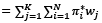^* (7)

where π_i^* is the inflation target, and i = 1, 2, 3, … N indicates the number of objectives that each country has had. w_j indicates the period of time that said objective has been maintained, thus j = 1, 2, 3, … K indicates the quarters. Details are given in Table 6.

Table 8. Average target inflation

Notes: US, Japan and EA have had an inflation target of 2% since the adoption of IT. ‘Q’ represents quarters. Source: Own elaboration.

3. Interbank Interest Rate Estimation

We estimate the regression by assuming that inflation is at its targeted level and the output gap is zero. The rationale behind this estimation approach stems from our objective of comparing periods during which the economy operated at its natural level.

After IT: (8)

Before IT: (9)

where the parameters are those that we obtain from the model, whereas the average target inflation level parameters (π^*) are the ones we estimate in Figure 2.

4. Elasticities for Inflation and Output

For reference purposes, we estimate the elasticities of inflation and the output gap in both periods (pre- and post-IT). The estimate is as follows (Table 4):

Elasticity of inflation = (10)

Elasticity of output gap = 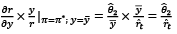(11)

where the only thing that changes is for both periods (estimate is obtained from Equations (11) and (12), is the growth rate of natural output for each country (Table 5).

Appendix B. Tables and Figures

Table 9. Results with IV estimation (Equation (1))

Notes: Standard errors are reported in parentheses. Asterisks denote statistical significance at the 1% (*), 5% (**), and 10% (***) levels. Standard errors were calculated by using the HAC robust estimator. The instruments used were the own lags of each variable. The Akaike Information Criterion (AIC) was used to determine the optimal number of lags, with a maximum of 12 lags (6 for the Euro Area to avoid rank issues). For individual countries: for Peru, we used 10 lags for inflation and 1 lag for the output gap; for Chile, we used 4 lags for the output gap and 10 lags for inflation; for Colombia, we used 10 lags for inflation and 5 lags for the output gap; for Mexico, we used 12 lags for inflation and 1 lag for the output gap; for Brazil, we used 2 lags for inflation and 3 lags for the output gap; for Canada, we used 9 lags for inflation and 1 lag for the output gap; for the U.K., we used 9 lags for inflation and 4 lags for the output gap; for the U.S., we used 10 lags for inflation and 4 lags for the output gap; for Japan, we used 5 lags for inflation and 1 lag for the output gap; and, for the Euro Area, we used 6 lags for inflation and 1 lag for the output gap.

Figure 3. Transition functions

Notes: Dynamic of logistic transition functions for each country are presented. These results are derived from the estimation of Equation (2).

Table 10. Robustness check

Notes: The dates before and after IT correspond to a specific date for each country. Standard errors are reported in parentheses. Asterisks denote statistical significance at the 1% (*), 5% (**), and 10% (***) levels. Standard errors were calculated by using the HAC robust estimator.