Ekonomika ISSN 1392-1258 eISSN 2424-6166

2025, vol. 104(1), pp. 30–47 DOI: https://doi.org/10.15388/Ekon.2025.104.1.2

Debt Trapped: Analysing the Impact of IMF on Economic Growth and Human Development in Highly Indebted Countries, with a Focus on Corruption

Doaa M. Salman Abdou*
October University for Modern Sciences and Arts, Cairo, Egypt
Email: dsalman@msa.edu.eg
ORCID: https://orcid.org/0000-0001-5050-6104

Ahmed Adel El-Ahmar
October University for Modern Sciences and Arts, Cairo, Egypt
Email: ahmed.adel38@msa.edu.eg
ORCID: https://orcid.org/0000-0002-9160-2001

Dina Youssri
German University, Cairo, Egypt
Email: Dina.elsayed@guc.edu.eg
ORCID: https://orcid.org/0000-0003-3516-3865

Jens Klose

THM Business School, Giessen, Germany
Email: jens.klose@w.thm.de
ORCID: https://orcid.org/0000-0001-6234-5272

Abstract. Being indebted represents significant risks associated with global financial instability in a world where financial stability hangs precariously between debt and economic growth. The International Monetary Fund (IMF) casts a critical eye over countries navigating the perilous seas of fiscal responsibility, aiming to improve their economic performance. Hence, evaluating the connection between IMF loans and sustainable growth in highly indebted countries is crucial. This study aims to examine the impact of IMF loans on real GDP and human development in a panel of the 13 most indebted countries from 1997 to 2020, by using pooled OLS and fixed-effect estimators. The article contributes to the existing literature in two ways. On the one hand, a broad set of human development indicators is analysed. On the other hand, corruption is incorporated into the analysis, explicitly measuring the simultaneous effects of IMF loans and corruption. It has been found that IMF loan growth tends to lower GDP growth, human development, and mortality. IMF loans often come with conditions that may lead to austerity measures. While these measures can negatively impact economic growth in the short term, they might also redirect resources toward social programs which improve health outcomes, thereby reducing mortality rates. When corruption is considered, a reduction in corruption leads to more effective IMF loans, increased human development, and decreased mortality even further. Therefore, it is recommended that IMF loans should always be accompanied with incentives to reduce corruption.
Keywords: IMF loans, HDI, indebted countries, corruption, economic growth, life expectancy, mortality, education.

_________

* Correspondent author.
Received: 17/09/2024. Revised: 21/11/2024. Accepted: 05/01/2025
Copyright © 2025 Doaa M. Salman Abdou, Ahmed Adel El-Ahmar, Dina Youssri, Jens Klose. Published by Vilnius University Press
This is an Open Access article distributed under the terms of the Creative Commons Attribution License, which permits unrestricted use, distribution, and reproduction in any medium, provided the original author and source are credited.

Introduction

Human development is widely recognized as one of the key drivers of a country’s economic growth. Improved education and health lead to the acquisition of skills, particularly the ability to innovate, which can boost economic growth. Moreover, human development enhances people’s choices and diversifies them in a way that enables them to lead longer, healthier, and more fulfilling lives. Given its importance, the United Nations has addressed human development extensively in its Sustainable Development Goals (SDGs), with seven of the 17 goals focusing on different aspects of human development, such as reducing poverty, improving health and education, and promoting gender equality. However, most countries fail to develop balanced debt management policies that can help them to achieve growth even if they receive external assistance from institutions such as the International Monetary Fund (IMF) and the World Bank (Elkhalfi et al., 2024).

The IMF plays a critical role in developing countries, where corruption can misdirect the use of IMF loans, with funds getting wasted on projects that do not actually benefit the country. This study aims to examine the impact of IMF loans on economic growth and human development in the most indebted countries. Some scholars have expressed concern that the engagement is a debt trap, a ruse towards modern neo-colonization and resource extinction in Africa. However, others have documented the significance of such investments in attaining SDGs (Bo et al., 2024)

This article extends previous research in the literature in two ways. First, it starts with measuring the effects of IMF loans on a broad set of dependent variables. These are, on the one hand, the real GDP growth as the common proxy for economic growth, and, on the other hand, the Human Development Index (HDI), secondary school enrollment, life expectancy, and mortality rate, which are used to measure human development. Second, a new dimension is added to the literature by adding corruption to the analysis. With this factor being considered, we can verify whether IMF loans have different effects in high- and low-corruption economies. This study focuses on the transmission channels and discusses various factors that might mediate the indebtedness-mortality link. For example, we note that higher levels of debt accumulation result in increased austerity. The following section discusses the literature review, followed by an overview of the data used. Finally, the results, conclusion and policy recommendations are outlined.

Literature Review

The classical school, in contrast with Keynesian economists, believed in the Government’s role in regulating the market and correcting imbalances through public borrowing as part of Government intervention in the economy to ensure upward economic evolution. They believed that accumulation of debt led to a crowding-out effect, thereby decreasing private investments, which deteriorated economic growth. The Debt Overhang Theory, established by Krugman in 1988, explains the situation in which the accumulated loans and debt make the country unable to repay them, thus decreasing its expenditure ability on public projects such as infrastructure, social programs, or financing the recurrent expenditure. In 1964, Gary Becker explored how education and training contribute to economic success, and explained why developed countries accumulate wealth while developing countries remain poor due to labour (under)productivity. The model states that a higher investment in capital per worker leads to a higher output, with investment per worker being the main variable positively impacting changes in capital per worker. Therefore, debt should be directed to finance education, improve infrastructure, and develop healthcare services so that to improve human capital and technology, which are considered the main sources for the country’s future income generation.

The effectiveness of IMF programs and loans on the countries receiving help has already been investigated extensively. This also holds, among other points, for the empirical response to economic growth and human development. Barro and Lee (2005) found that IMF loans reduce economic growth rates in their sample of 130 countries between 1975 and 1999. Meanwhile, Bird and Rowlands (2017) discovered that the impact of IMF loan programs on economic growth in low-income countries is generally positive, however, it depends on the country’s performance, debt and aid dependency, IMF resources, and the recent history of IMF engagement. Later, Hackler et al. (2020) estimated empirically for 93 countries between 2000 and 2014 what effects the compliance to IMF loan conditions tends to have on economic growth. The authors established that meeting the IMF conditions can change the economic growth rate either way depending on the nature of the condition.

Siddique et al. (2021), by using panel data covering 70 countries during the period of 1980–2018, determined that IMF loans had a positive impact on economic growth for upper-middle-income countries. Kuruc (2022) used a synthetic control analysis of IMF interventions in 399 different crisis periods between 1970 and 2013. With this approach, he could show that IMF programs led to higher economic growth than in a situation without a program in place.

Another strand of literature focuses on the role of IMF programs for human development. Easterly (2003), by using data from 1980 to 1998, established that IMF and World Bank programs have no significant direct effect on poverty rates. However, he found that the growth elasticity of poverty is significantly negative, which means that the poor segment of the population benefits less from economic expansion under a program. Muhamed and Gaas (2016) discovered that IMF programs had a negative impact on human development in developing countries. Bird et al. (2021) determined that IMF programs did not significantly increase poverty or income inequality by using a sample of 48 countries in the years ranging from 1990 to 2015. Stubbs et al. (2021) focused on the austerity policies often associated with IMF programs and their effects on poverty and income inequality. In a sample covering 79 countries between 2002 and 2018, they ascertained that stricter austerity policies in IMF programs led to more poverty and higher income inequality.

Biglaiser and McGauvran (2022) found that IMF loans reduce human development in developing countries in a sample of 81 countries between 1986 and 2016. This result holds in particularly concerning poor nations. Corruption is a factor that may affect the effectiveness of IMF loans and is associated with lower growth and more poverty. A recent strand of the literature emphasizes the importance of e-government in combating corruption and promoting transparency (Seiam and Salman, 2024). Apeagyei et al. (2024) showed that many sub-Saharan African countries suffer from poverty and income inequality, deteriorating public health, educational outcomes, increasing child mortality, and corruption. The IMF provides financial assistance to countries facing balance of payments problems, and numerous sub-Saharan nations have engaged with the IMF through various lending programs.

This study contributes to the ongoing discussion on the effectiveness of IMF loans. First, we are one of the few studies that estimate the effects of IMF loans on economic growth and human development simultaneously. Second, to the best of the researchers’ knowledge, they are the first to investigate the role of corruption in IMF programs and their effect on growth and development. Third, we focus on a unique database with 13 highly indebted countries in the years ranging between 1997 and 2020. The study’s main hypotheses are:

• IMF loans tend to lower the GDP growth and human development (e.g., life expectancy, education) in the short term.

• The effectiveness of IMF loans improves when corruption is reduced, thus leading to enhanced human development and decreased mortality.

Methodology and Data

Our panel dataset is comprised of 13 countries which received IMF loans during the period from 1997 to 2020. These countries are Angola, Argentina, Ecuador, Egypt, Ghana, Ivory Coast, Kenya, Morocco, Nigeria, Pakistan, South Africa, Tunisia, and Ukraine. For each of these countries, we gathered data on five dependent variables, representing measures of either economic growth or human development. Economic growth is approximated by the real gross domestic product (GDP). Additionally, we incorporated two of the three sub-indices used in the HDI calculation. Thus, the second measure represents the share of secondary school enrollment, while the third measure represents life expectancy. The fourth measure is the mortality rate, which is expected to negatively correlate with life expectancy.

As for independent variables, we collected data on the two primary variables of interest: the amount of money received through IMF loans, and the country’s corruption index. For the corruption index, we utilized the Corruption Perception Index issued by Transparency International¹. It is of importance to note that an increase in this index indicates a reduction in corruption within the country. Furthermore, we included a set of six additional control variables in all the estimation equations. These include Gross capital formation (GCF), Government expenditures on education (as a percentage of the total Government expenditures), trade in services, consumer price index, foreign direct investments (FDI), and the size of the population. To ensure the stationarity of the underlying time-series data, all the variables were transformed into growth rates. For example, the price index was transformed into the inflation rate. Descriptive statistics along with unit root tests for all variables are presented in Table 1 in the Appendix.

Correlation Analysis

The analysis reveals a strong positive correlation between IMF loans and GDP in the studied countries, thereby indicating that as IMF loans increase, GDP also rises. There are several other significant correlations: a weak negative correlation exists between the mortality rate and both IMF loans and corruption. Secondary school enrollment shows a weak positive correlation with GDP, IMF loans, and corruption, along with a strong negative correlation with the mortality rate. Human development exhibits a weak positive correlation with GDP, IMF loans, and corruption, but strong negative correlations with the mortality rate and positive correlations with secondary school enrollment. Government expenditure on education has weak negative correlations with GDP and IMF loans, but weak positive correlations with corruption, mortality, secondary school enrollment, and human development. Inflation negatively correlates with GDP, corruption, secondary school enrollment, and human development. Foreign direct investment (FDI) shows weak negative correlations with GDP, IMF loans, secondary school enrollment, and human development, while strongly correlating positively with inflation. Gross capital formation has weak negative correlations with GDP and IMF loans, and trade in services negatively correlates with GDP. Population growth is weakly negatively correlated with GDP, IMF loans, corruption, secondary school enrollment, and Government expenditure. For detailed correlations, refer to Table 2 in the Appendix.

Estimation Methodology

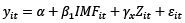
The study used a cross-dependence test to determine the suitability of pooled versus random effects models. The model includes five dependent variables, and employs two estimation methods: pooled ordinary least squares (OLS), assuming a common intercept for all the countries under analysis, and fixed-effects estimation, allowing for individual country intercepts. Detailed findings are presented in Tables 3 to 7 in the Appendix. Two different types of estimation are employed: first, a pooled ordinary least squares (OLS) estimation, which assumes that all countries have the same intercept (see Equation (1)); and second, a fixed-effects estimation, which allows each country to have an individual intercept (see Equation (2)).

(1)

(2)

In both equations, the index i signals the country and t stands for the time period (years in our case). y denotes one of the five dependent variables (GDP, HDI, School, Life, or Mortality). α represents the common or individual intercept, while β₁ and γ_x are the coefficients for IMF loans and the control variables (GCF, Education, Trade, Price, FDI and Population), respectively. It should be noted that x ranges from 1 to 6 in line with the responses to be estimated for each of the six control variables. Finally, ε_it measures the error term.

(3)

(4)

In Equations (1) and (2), the effect of corruption is not included. This is deliberate to first demonstrate the overall effects of IMF loans on the dependent variables. In a subsequent step, however, we incorporate corruption. This is done in two ways: firstly, by adding corruption as an additional regressor. Secondly, by adding the product of IMF and corruption, we demonstrate how the dependent variable changes concerning IMF loans and changes in corruption. Equations (3) and (4) depict these adjusted specifications using pooled OLS and fixed-effects, respectively.

Results

This section presents and discusses the empirical results. It begins with the specifications that do not consider the influence of corruption, as outlined in Equations (1) and (2). The results are presented in Table 8.

Table 8. Baseline results

Notes. C stands for the constant (only for pooled OLS. Fixed effects constants are available from the authors upon request), N denotes the number of observations, whereas Adj. R² is the adjusted R² value. All other abbreviations are explained in the main text. Standard errors are given in parentheses, ***/**/* stands for the significance of the coefficients at 99%, 95% and 90% levels, respectively.

The response of GDP growth was found to be significantly negative in both specifications (2.1 and 2.2), although the effect tends to be small. This suggests that an increase in IMF loans is associated with lower economic growth in the short term, possibly due to the stringent reform packages typically associated with IMF support. This finding reinforces the results of previous studies by Barro and Lee (2005). However, there are three exceptions worth noting. Firstly, gross capital formation shows a positive and significant effect on economic growth. A one percent increase in gross capital formation leads to an increase of 0.15% in economic growth. This result is logical as gross capital formation is a component of GDP. Secondly, GDP growth reacts negatively to an increase in the price index, thereby indicating that higher inflation rates reduce economic growth, with everything else being equal. This result is expected as increased prices diminish product demand. Thirdly, population growth appears to positively influence economic growth, as expected, thus indicating that countries with larger populations tend to produce more goods and services.

Concerning the response to HDI growth (2.3 and 2.4), the results suggest a weakly negative effect of IMF loan growth on HDI growth, which becomes significant in the pooled OLS Equation (2.3). This implies that, at least in the short term, IMF loans and the austerity programs often associated with them tend to reduce human development. This finding is consistent with previous studies by Muhamed and Gaas (2016) and Biglaiser and McGauvran (2022). The control variables tend to be predominantly significant in these specifications. Gross capital formation (GCF) growth exhibits a robust positive effect on HDI growth, which is reasonable as investments may occur in sectors that enhance human development, such as education or healthcare. Unsurprisingly, the response of HDI growth to the Government’s schooling expenditure increases is significantly positive, as this directly contributes to human development. Additionally, increasing international trade growth was found to increase HDI growth, likely due to the broader range of goods and services available via imports, which can improve access to items such as medication. Interestingly, the inflation rate initially appears to have a significantly positive effect on HDI growth in the pooled OLS Equation (2.3). This result is puzzling, as one might expect a negative response, given that higher inflation rates could deter investments aimed at improving human development. However, the significance diminishes once fixed effects have been incorporated into the estimation (2.4). Finally, according to the results, human development growth increases with population growth. One possible explanation for this is that an increasing population necessitates the development of critical infrastructure, leading to improvements in healthcare and education systems.

When examining the first factor contributing to HDI, which is School growth, we find that growth in IMF loans tends to have no effect (3.5 and 3.6). This suggests that, in the short term, an IMF credit does not significantly contribute to the development or improvement of the schooling system. This finding aligns with the expectations, as establishing or enhancing a schooling system is typically a medium- to long-term endeavour. Regarding the control variables, we observe similar significantly positive reactions to school growth as we found concerning HDI growth for variables such as gross capital formation (GCF), trade, and population growth. Thus, it can be inferred that HDI growth, particularly in terms of school growth, is partly driven by these factors. Moreover, we now find that the response of school growth to the inflation rate has the expected significantly negative impact, as higher prices tend to discourage investments in the schooling system. However, the result regarding Government expenditures on education is puzzling, as it is found to have a significantly negative effect on school growth. One possible explanation is that the effects of these expenditure increases do not materialize immediately, and may even hinder schooling improvement due to factors such as renovations of school buildings.

Lastly, we find a significantly negative effect of foreign direct investment (FDI) growth on school growth. One explanation for this could be that, in many of the countries under investigation, which are predominantly low-income countries, FDI investments are mainly directed towards sectors requiring unskilled labour. Consequently, an increase in FDI may lead to a greater demand for unskilled workers, thus prompting individuals to forgo or reduce their education. When examining the effects on growth in life expectancy, the results are presented in columns 2.7 and 2.8 of Table 8. Finally, when examining the response of mortality growth (2.9 and 2.10), we find the expected significantly negative response, which corresponds to the significantly positive effect we found regarding growth in life expectancy. This suggests that, as the population grows, mortality rates tend to decrease, which is consistent with the notion that larger populations may lead to an improved access to healthcare and other life-saving resources.

The coefficients for the impact of IMF loans on GDP growth and HDI growth are notably small, thereby suggesting that while there is a statistically significant relationship, its practical significance may be limited. For instance, a negative coefficient for GDP growth implies that an increase in IMF loans leads to a slight decline in growth rates, which could be critical in economies where even marginal declines can have adverse effects on the overall economic stability (3.1 and 3.2). The responses of the control variables are largely unchanged from those observed in Table 9, thus indicating that the explanations provided there remain valid.

Table 9. Results of the main contribution; corruption is added to the estimation equations

Notes. C stands for the constant (only for pooled OLS. Fixed effects constants are available from the authors upon request), N denotes the number of observations, and Adj. R² is the adjusted R² value. All other abbreviations are explained in the main text. Standard errors are given in parentheses, ***/**/* stands for the significance of the coefficients at 99%, 95% and 90% levels, respectively.

Given the short-term nature of these coefficients, it is crucial to analyse whether these effects change over a longer horizon. The immediate negative impact on GDP growth suggests that austerity measures associated with IMF loans may hinder growth in the short run, potentially leading to a cycle of dependency on loans without fostering sustainable development.

When incorporating corruption into the equations, the effects on HDI growth manifest some change (3.3 and 3.4). Firstly, no significant effect of IMF loan growth on HDI growth is observed any more. Secondly, if an increase in IMF loans is accompanied by a reduction in corruption, this has significantly positive effects on HDI growth. Thirdly, the effects of the additional control variables remain broadly unchanged compared to those observed in Table 9. Finally, concerning mortality growth (3.9 and 3.10), we still find the significantly negative influence of IMF loan growth, as observed in Table 9. Moreover, this effect is strengthened if IMF loans are accompanied by a reduction in corruption. This underscores the importance of accompanying IMF loans with obligations or incentives to reduce corruption, as it can have a significant impact on mortality rates.

Random Effects Model with Control of Corruption

The analysis of the real GDP model reveals several key findings: a 1% increase in IMF loans is associated with a 0.129% increase in real GDP, which is significant at the 1% level. Enhancing the control of corruption by one unit correlates with a substantial 31% increase in real GDP, which is also significant at the 1% level. A one-unit increase in gross capital formation (GCF) results in a 0.702% increase in real GDP, which is significant at the 5% level. The inflation rate shows significance at a 10% level.

The Human Development Index (HDI) model indicates that a 1% increase in IMF loans leads to a decrease in HDI by 0.00022 units, which is significant at the 1% level. Gross capital formation (GCF) and education are significant at the 5% level. If all independent variables are held constant at zero, HDI is projected to be 0.198. In the mortality rate model, a 1% increase in IMF loans correlates with a 0.04828 units reduction in the mortality rate (significant at the 1% level). A one-unit increase in corruption control results in a 6.636 units decrease in the mortality rate (significant at the 5% level).

Table 10. Estimated random effects model with control of corruption

* p<0.10; ** p<0.05; *** p<0.01

Source: based on the author’s calculations.

Generalized Method of Moments (GMM) with Control of Corruption

The model exhibits dynamic characteristics, showing a significant positive effect of the previous year’s GDP on the current GDP. Specifically, a 1% increase in last year’s GDP leads to a 0.989% increase in the current GDP. When independent variables are set to zero, the estimated real GDP is 0.340. Regarding Human Development Index (HDI), IMF loans positively impact it; a 1% increase in loans corresponds to a 0.002% increase in HDI, which is converted to 0.00002 units.

The mortality rate model shows dynamic characteristics, where the previous year’s mortality rate significantly influences the current year’s rate. Specifically, a 1-unit increase in the last year’s rate results in a 0.946-unit increase in the current year’s rate at the 1% significance level. Additionally, IMF loans have a significant negative effect on mortality; a 1% increase in loans leads to a 0.140% decrease in the mortality rate, also significant at the 1% level. In the school enrollment model, the previous year’s enrollment positively affects the current year’s enrollment. A 1-unit increase in last year’s enrollment results in a 0.474-unit increase in the current year’s enrollment at the 1% significance level. Furthermore, a 1% increase in IMF loans correlates with a 1.587% increase in school enrollment, significant at the 5% level.

Table 11. Generalized method of moments (GMM) with control of corruption

* p<0.05; ** p<0.01

Source: based on the author’s calculations.

Conclusion

In this paper, we empirically estimated the effects of IMF loans on economic growth and human development, by using various indicators. Additionally, we incorporated the role of corruption into the analysis to explore whether IMF loans become more or less effective under different levels of corruption. The small coefficients indicate that the influence of IMF loans on economic indicators is subtle and may require further investigation. This raises questions about the effectiveness of IMF interventions and whether they are sufficient to stimulate substantial economic growth in highly indebted countries. Policymakers should consider these findings when designing loan conditions and reform packages to ensure that they are really impactful.

The results suggest that IMF loans negatively impact economic growth while reducing mortality rates. This dual effect raises concerns for policymakers, as short-term austerity measures linked to IMF loans can hinder economic activity, potentially leading the public to blame the IMF for downturns. To maintain public support for the necessary reforms, the IMF should consider easing down short-term consolidation efforts so that to foster growth. Additionally, the interaction between IMF loans and corruption indicates that Human Development Index (HDI) growth improves with both IMF loans and reduced corruption, while further lowering mortality rates. This suggests that IMF programs should prioritize anti-corruption measures in order to enhance human development.

The study focuses on short-term effects, highlighting the need for further research into the medium- to long-term impacts of IMF loans and corruption. Future studies could utilize panel vector autoregression to explore these dynamics, although data limitations in developing countries may pose challenges. Such research would be crucial for understanding the lasting impacts of IMF loans on economic and human development.

Policy Recommendations

• The findings urge the IMF to re-evaluate the conditions attached to loans. If the coefficients remain small, it may suggest that the current policies are ineffective in promoting growth. The IMF might need to incorporate more flexible and supportive measures that would facilitate growth while still addressing the fiscal challenges of borrowing countries.

• IMF loans should always be accompanied with measures tailored to reduce corruption. Lower corruption levels increase the effectiveness of these loans, especially in improving human development and reducing mortality.

• The IMF should consider relaxing short-term austerity measures to help indebted countries maintain economic growth while implementing the necessary reforms.

Limitations

One limitation of this study is the relatively small sample size of 13 countries, which may affect the robustness and generalizability of the findings. Additionally, the sample is unbalanced, potentially introducing bias and limiting the ability to draw definitive conclusions about the relationships among the variables.

Data Availability Statement

All data will be made available upon reasonable request.

References

Alia, H., Farooq, F., Sheikh, M., and Perveeen, A. (2022). Education, Human Capital, and Endogenous Growth Nexus: Time Series Evidence from Pakistan. Review of Education, Administration and Law (REAL), 5(2), 109–121. https://doi.org/10.47067/real.v5i2.223

Amoh, J. K., Abdul-Mumuni, A., Penney, E. K., Muda, P., & Ayarna-Gagakuma, L. (2024). Corruption and external debt nexus in sub-Saharan Africa: a panel quantile regression approach. Journal of Money Laundering Control, 27(3), 505–519. https://doi.org/10.1108/JMLC-07-2023-0125

Apeagyei, A. E., Lidral-Porter, B., Patel, N., Solorio, J., Tsakalos, G., Wang, Y., & Nonvignon, J. (2024). Financing health in sub-Saharan Africa 1990–2050: Donor dependence and expected domestic health spending. PLOS Global Public Health, 4(8), e0003433. https://doi.org/10.1371/journal.pgph.0003433

Balima, W. H., Sokolova, A. (2021). IMF programs and economic growth: A meta-analysis. Journal of Development Economics, 153, 102741 https://doi.org/10.1016/j.jdeveco.2021.102741

Barro, R. J. and Lee, J. W. (2005). IMF programs: Who is chosen and what are the effects? Journal of Monetary Economics, 52, 1245–1269. https://doi.org/10.1016/j.jmoneco.2005.04.003

Becker, G. S. (1964). Human capita. Chicago: University of Chicago Press.

Biglaiser, G., and McGauvran, R. (2022). The effects of IMF loan conditions on poverty in the developing world. Journal of International Relations and Development, 806–833. https://doi.org/10.1057/s41268-022-00263-1

Bird, G., and Rowlands, D. (2017). The Effect of IMF Programmes on Economic Growth in Low Income Countries: An Empirical Analysis. The Journal of Development Studies, 53(12), 2179–2196. https://doi.org/10.1080/00220388

Bird, G., Qayum, F., and Rowlands, D. (2020). The effects of IMF programs on poverty, income inequality and social expenditure in low-income countries: an empirical analysis. Journal of Economic Policy Reform, 24(2): 170–188. https://doi.org/10.1080/17487870.2019.1689360

Bo, H., Lawal, R., & Sakariyahu, R. (2024). China’s infrastructure investments in Africa: An imperative for attaining sustainable development goals or a debt-trap? The British Accounting Review, 101472. https://doi.org/10.1016/j.bar.2024.101472

Easterly, W. (2003). IMF and World Bank Structural Adjustment Programs and Poverty, in Dooley, M. P. and Frankel, J. A. Managing Currency Crises in Emerging Markets, chapter 11, University of Chicago Press. https://doi.org/10.7208/9780226155425-013

Elkhalfi, O., Chaabita, R., Benboubker, M., Ghoujdam, M., Zahraoui, K., El Alaoui, H., ... & Hammouch, H. (2024). The impact of external debt on economic growth: The case of emerging countries. Research in Globalization, 100248. https://doi.org/10.1016/j.resglo.2024.100248

Hackler, L., Hefner, F., and Witte, M. D. (2020). The Effects of IMF Loan Condition Complinace on GDP Growth, The American Economist, 65(1), 88–96. https://doi.org/10.1177/056943451983

International Monetary Fund. (2000). IMF-Supported Programs and the Poor: The Experiences of Low-Income Countries. Retrieved May 15, 2023, from https://www.imf.org/external/pubs/ft/pam/pam52/3.htm

Kuruc, K. (2022). Are IMF rescue packages effective? A synthetic control analysis of macroeconomic crises, Journal of Monetary Economics, 127, 38–53. https://doi.org/10.1016/j.jmoneco.2022.02.002

Roberts, R. O. (1942). Ricardo’s theory of public debts. Economica, 9(35), 257–266. https://doi.org/10.2307/2549539

Siddique, I., Hayat, M., Naeem, M., Ejaz, A., Spulbar, C., Birau, R., and Calugaru, T. (2021). Why Do Countries Request Assistance from International Monetary Fund? An Empirical Analysis. Journal of Risk and Financial Management. https://doi.org/10.3390/jrfm14030098

Seiam, D. A., & Salman, D. (2024). Examining the global influence of e-governance on corruption: a panel data analysis. Future Business Journal, 10(1), 29. https://doi.org/10.1186/s43093-024-00319-3

Stubbs, T., Kentikelenis, A., Ray, R. and, Gallagher, K. P. (2022). Poverty, Inequality, and the International Monetary Fund: How Austerity Hurts the Poor and Widens Inequality. Journal of Globalization and Development, 13(1), 61–89. https://doi.org/10.1515/jgd-2021-0018

Appendix

Table 1. Descriptive statistics and unit root tests

Notes. Panel unit root test testing for a common unit root as introduced by Levin et al. (2002). For the unit root tests, we show the corresponding p-values in parentheses.

Table 2. Pairwise correlation

Source: based on the author’s calculations

Table 3. Cross dependence test

Table 4. Hausman Test

Hausman (1978) specification test

Table 5. Normality Test

Table 6. VIF Test

Table 7. Breusch-Pagan for Heteroscedasticity