Ekonomika ISSN 1392-1258 eISSN 2424-6166

2025, vol. 104(2), pp. 59–77 DOI: https://doi.org/10.15388/Ekon.2025.104.2.4

The Interplay Between Economic Policy, Oil Price and Economic Growth in Malaysia

Siow Xiu Yun
Universiti Malaysia Sabah
Jalan UMS, 88400 Kota Kinabalu, Sabah, Malaysia
Email: XIU_YUN_SIOW_MB22@iluv.ums.edu.my
ORCID: https://orcid.org/0009-0007-5884-562X

Wong Hock Tsen*
Universiti Malaysia Sabah
Jalan UMS, 88400 Kota Kinabalu, Sabah, Malaysia
Email: htwong@ums.edu.my
ORCID: https://orcid.org/0000-0001-5789-2511

Abstract. This study examines the interactions among the oil price, Government expenditure, money supply, real effective exchange rate, and Gross Domestic Product (GDP) across Malaysia’s finance, retail and wholesale, manufacturing, agriculture and overall sectors by using a Structural Vector Autoregression (SVAR) model. The variance decomposition has revealed an increasing interconnectedness among the variables over time, with external factors such as global commodity prices and fiscal policies becoming more significant in shaping sectoral dynamics. The impulse response function analysis highlighted sector-specific variations: the finance and retail sectors predominantly exhibited positive responses to the oil price and GDP shocks, while the agriculture sector showed mixed responses, reflecting its reliance on external and policy-driven factors. The manufacturing sector displayed sensitivity to monetary conditions, while the overall sectoral trends suggested the ability to absorb shocks effectively. The findings highlight the need for sector-specific policies so that to enhance Malaysia’s economic resilience and achieve SDG 8, advising policymakers to adopt adaptive fiscal and monetary measures, strengthen agricultural resilience, and promote diversification in the retail and manufacturing sectors for inclusive and sustainable growth.
Keywords: Oil price, economics policy, real effective exchange rate, gross domestic product, structural vector autoregression, impulse response.

_________

* Correspondent author.

Received: 05/11/2024. Revised: 30/12/2024. Accepted: 22/03/2025
Copyright © 2025 Siow Xiu Yun, Wong Hock Tsen. Published by Vilnius University Press
This is an Open Access article distributed under the terms of the Creative Commons Attribution License, which permits unrestricted use, distribution, and reproduction in any medium, provided the original author and source are credited.

Introduction

The interplay among the oil price, Government expenditure, money supply, the real effective exchange rate, and the Gross Domestic Product (GDP) is pivotal for understanding the economic dynamics of resource-endowed nations, including Malaysia. Notably, as a major oil-exporting nation, Malaysia’s economy remained highly susceptible to the global oil price fluctuations, which significantly affected fiscal revenues and public spending (Kriskkumar et al., 2022). Against this backdrop, fiscal and monetary policies emerged as critical mechanisms to stabilise growth and bolster its economic resilience (Wang et al., 2023). Specifically, the oil price, as a primary driver of the Government revenue, directly influenced fiscal policy and public expenditure decisions (Abubakar et al., 2023). Concurrently, the money supply played a central role in shaping inflation, interest rates and investment, while the exchange rate reflected the international trade competitiveness, thereby impacting the balance of payments and the overall economic output (Lal et al., 2023).

Malaysia faced challenges in achieving macroeconomic stability while pursuing SDG 8 – Decent Work and Economic Growth. The -0.8% GDP growth in 2022 highlighted post-pandemic economic struggles, while labour rights issues, such as modern slavery, affecting 6.3 per 1,000 people, raised concerns. However, the financial inclusion improved, with 88.4% of adults having access to financial services by 2021. Projections for 2024 suggested a recovery in the labour market, with an estimated unemployment rate of 3.6%. Despite this, issues like weak labour rights enforcement (0.58/1 in 2022) and work-related accidents, along with the modern slavery in imported goods, require urgent policy attention.

This study’s findings revealed that Malaysia’s finance sector was particularly vulnerable to external shocks, with the oil price, Government expenditure, and money supply collectively accounting for over 68% of GDP variance by the tenth period. This finding underscored the imperative for targeted fiscal and monetary policies to enhance the country’s economic resilience and foster its sustainable growth.

This objective of this study is to analyse the interrelationships of the oil price, Government expenditure, money supply, real effective exchange rate, and sectoral GDP in Malaysia, by using the Structural Vector Autoregression (SVAR) model. SVAR enables the identification and estimation of dynamic interactions between the variables, capturing both short- and long-term effects while accounting for their structural interdependencies. This study not only contributed to policymaking in alignment with SDG 8 but also addressed critical issues such as labour rights and financial inclusion. By doing so, it provided actionable policy recommendations aimed at supporting sustainable economic development and improving labour conditions.

Based on the currently existing literature, this study hypothesised that the oil price has a mixed effect on economic growth, with some studies showing a positive relationship (Taghizadeh-Hesary et al., 2019) and others indicating a negative one (Kriskkumar et al., 2022). It has also been posited that the Government expenditure positively impacts the GDP growth (Dudzevičiūtė et al., 2018), even though some studies report a negative effect (Cenc, 2022; Tan et al., 2020). Additionally, it has been hypothesised that the money supply and the Real Effective Exchange Rate (REER) positively influence economic growth (Mandler et al., 2022; Zhu et al., 2022), while other studies suggest a negative relationship with REER (Sami and Taiwo, 2023).

Ultimately, this research elucidates the transmission mechanisms that underpinned economic growth and stability, while offering valuable insights for policymakers. By aligning with SDG 8, it underscores the importance of promoting decent work and economic growth while addressing critical labour-related challenges. Consequently, this study contributes to the broader discourse on sustainable economic development in Malaysia, while offering practical policy interventions to enhance resilience and inclusivity.

This study is organised into five sections: Section 1 provides an introduction to the topic, Section 2 presents a review of the relevant literature, Section 3 outlines the data sources and the methodology employed, Section 4 discusses the empirical results, and Section 5 offers a discussion of the findings, along with policy recommendations and suggestions for future research directions.

Literature Review

The interconnection of the oil price, Government expenditure, money supply, the real effective exchange rate, and GDP is a key research focus, particularly in resource-rich economies like Malaysia. These dynamics are vital for fostering economic growth and guiding effective policymaking, especially given Malaysia’s status as an oil-exporting nation.

Notably, studies on oil price fluctuations reveal differing impacts on GDP across regions. For instance, in the European Union, Raduzzi and Ribba (2020) observed that oil price shocks significantly influenced business cycle fluctuations, thus underscoring their critical role in economic stability. Moreover, Van et al. (2019) highlighted that the oil price volatility adversely affected economic growth in OECD nations. However, Charfeddine et al. (2020) noted a minimal impact of the declining oil price on the United States’ GDP growth. In contrast, developing countries experienced more nuanced effects. For example, Kriskkumar et al. (2022) found that oil price fluctuations directly influenced the economic growth in Malaysia. Similarly, Taghizadeh-Hesary et al. (2019) reported that oil price shocks benefited oil-exporting economies directly, while having mixed indirect effects on oil-importing nations in the EU. Interestingly, Taghizadeh-Hesary et al. (2019) argued that GDP in the European Union did not align with other economic measures, thereby suggesting a more complex dynamic.

Furthermore, the role of the Government expenditure in economic growth has also received significant attention. For instance, Dudzevičiūtė et al. (2018) identified a strong positive relationship between the Government spending and economic growth in the EU countries. By contrast, Cenc (2022) revealed a significant negative relationship between the Government expenditure and economic growth across the European Union nations. In the case of Ghana, Poku et al. (2022) found that the Government expenditure positively correlated with economic growth. Interestingly, Al Jabri et al. (2022) demonstrated that the Government expenditure in Oman was not directly influenced by the oil price. For Malaysia, Tan et al. (2020) highlighted that the Government spending negatively impacted economic growth, whereas the monetary policy was found to be more effective in stimulating the economy.

Turning to monetary policy, Mandler et al. (2022) observed that the real output and money supply in Germany responded more strongly to monetary interventions compared to other countries. In addition, Sami and Taiwo (2023) found that exchange rate fluctuations significantly affected GDP in Nigeria. Similarly, Abdullah et al. (2022) demonstrated that exchange rate movements had a balanced impact on the money supply in Malaysia. Moreover, Zhu et al. (2022) noted that an undervalued currency boosted exports, thus significantly contributing to economic growth in Asian economies.

Building on this body of literature, the present study addresses a critical gap by exploring the complex interactions among these variables within specific economic sectors in Malaysia, an area that has received limited attention in previous research which primarily focused on the overall GDP. By examining sector-specific dynamics across the finance, retail and wholesale, manufacturing and agriculture sectors, this study provides a more granular understanding of how macroeconomic variables, such as the oil price, Government expenditure, money supply, real effective exchange rates and GDP, affect different parts of the economy. This sectoral focus is particularly beneficial for developing targeted policies which cater to the distinct needs and challenges of each particular sector, which would be overlooked in broader, aggregated analyses. Crucially, the research findings contribute to Sustainable Development Goal (SDG) 8 by enabling the formulation of effective strategies to support sustainable economic development and improve the labour conditions within specific industries. This approach not only enriched academic discourse by highlighting the importance of sector-specific analysis but also had practical implications for managing economic stability and fostering growth in resource-rich economies. By addressing this gap, this study offers valuable insights for policymakers and practitioners, ultimately helping to shape more informed, effective economic strategies tailored to each sector’s unique needs and challenges.

Data and Methodology

Data

This study aims to explore the interconnections between the oil price, Government expenditure, money supply, real effective exchange rate, and GDP across the finance, retail, manufacturing, agriculture and overall sectors in Malaysia, by using the Structural Vector Autoregressive (SVAR) model. This study uses quarterly data from Q1 2000 to Q3 2024. The selected timeframe encompasses significant economic and policy changes in Malaysia, including the global financial crisis of 2008 and the economic downturn triggered by the COVID-19 pandemic, which emerged in December 2019. The data sources include Bloomberg, the official portal of the Ministry of Economy and the Department of Statistics Malaysia official website. The Oil price (OIL) was measured by using the West Texas Intermediate (WTI) crude oil first contract, quoted in USD per barrel. The Government expenditure was represented by the total Government spending in Malaysian Ringgit (RM). Money supply (M2) was captured by the monthly M2 money supply in RM, reported year-over-year. The Real Effective Exchange Rate (REER) was based on the USD/MYR exchange rate, expressed as a dimensionless index. The Gross Domestic Product (GDP) was measured as the overall GDP, including finance, retail and wholesale, manufacturing, agriculture and overall sectors, in RM and adjusted for inflation.

The real values for oil, Government expenditure, money supply and GDP were calculated by dividing the nominal values by the Consumer Price Index (CPI), which adjusts for inflation. The CPI, reported as an index with the base year set to 100, captures price level changes over time. This adjustment yielded real values reflecting true economic conditions in constant prices. All variables were then transformed into natural logarithms to standardize the data for econometric analysis.

Econometric Framework

This study employs the Structural Vector Autoregression (SVAR) model, as proposed by Sims (1980), which facilitates the identification of structural shocks arising from specific macroeconomic variables and allows for the analysis of their impacts on other economic indicators. SVAR models are particularly effective for examining how a system responds to unexpected changes, whereas simultaneous equation models are more suitable for simulating policy outcomes (Crispín et al., 2023).

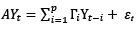
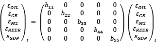
Utilisation of the SVAR model enables the analysis of macroeconomic shocks, such as oil price fluctuations, by decomposing them into components, including supply and demand shocks. The model incorporates critical variables such as the oil price, Government expenditure, money supply, the real effective exchange rate, and gross domestic product for various sectors, thereby assessing their sensitivity to these shocks. The SVAR model can be represented mathematically as follows (Manning, 2024; Yildirim and Guloglu, 2024):

(1)

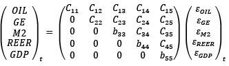
where Y_t is a vector of endogenous variables, A is the contemporaneous relationship matrix, Γ_i represents the lagged coefficient matrices, and ε_ₜ denotes the vector of structural shocks. Vector Y_t encompasses OIL, GE, M2, REER and GDP. In A, the diagonal elements are set to 1, while the off-diagonal elements, –α_ij , represent the contemporaneous relationships among the variables. The lagged coefficient matrices Γ_i capture the effects of the past values of the variables on the current values of Y_t. Each element –r_ij in Γ_i reflects the influence of the past value of the j – th variable on the i – th variable at lag i. Finally, ε_ₜ is a vector of structural shocks, with each element representing an unexpected disturbance in a specific variable, such as an oil price shock or a sudden change in the Government expenditure. The SVAR model is constructed for the endogenous variables OIL, GE, M2, REER and GDP to examine the economic shock effects as follows (Onafowora and Owoye, 2019; Sims, 1980):

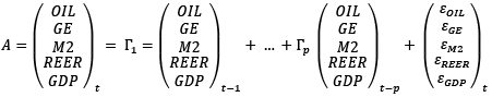(2)

As stated by Leng (2013), the Cholesky decomposition (Ω = P × P′) was performed on the variance and covariance matrix Ω of the structural impact term εₜ in Model 4, as outlined below:

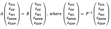(3)

The economic analysis of Malaysia includes five endogenous variables: OIL, GE, M2, REER and GDP across various sectors. Restrictions are used to better identify the model and to reflect the relationships between the different variables. These restrictions can be classified into two types. Short-term restrictions focus on the immediate relationships between the variables if one variable does not instantly affect another in the same period. For example, it may be assumed that the Government spending does not immediately respond to changes in the oil price or the money supply within the same timeframe. In contrast, long-term restrictions address how variables influence each other over an extended period. These assumptions suggest that certain relationships, such as between the Government spending and GDP, remain stable and maintain a consistent proportion over the long run. Such restrictions are crucial because they enhance the reliability of the Structural Vector Autoregressive (SVAR) model, making it more effective at estimating the interactions among macroeconomic variables. As highlighted by Nach and Ncwadi (2024), Sui et al. (2024), and Trabelsi (2024), application of both short-term and long-term restrictions enables the model to more accurately capture and explain the interrelationship of the variables.

The first restriction applied to the model was the short-term restriction. The short-term restrictions were added to the research model based on the relevant economic theories. We initially assume that OIL in the current period does not change with fluctuations in GE, M2, REER and GDP within the same period. This assumption suggests that OIL may be more significantly influenced by economic effects from previous periods and the anticipated future economic shocks. Consequently, the influencing factors in constraint A are set as α12 = α13 = α14 = α15=0

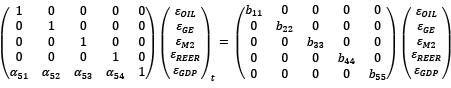(4)

The first restriction applied to the model was a short-term one. These short-term restrictions were used in the research model based on the relevant economic theories. The influencing factors in constraint A are set as α₁₂ = α₁₃ = α₁₄= α₁₅ = 0. Secondly, it is posited that the Government expenditure does not change with the money supply and the real effective exchange rate in the current period, which implies that there are lagged effects of the money supply and the real effective exchange rate on the Government expenditure, thus α₂₃ = α₂₄ = 0.

Finally, the premise that the money supply does not change with the real effective exchange rate in the current period suggests that there is a specific lagged effect of the real effective exchange rate, which means that α₃₄ = 0.

(5)

The second restriction applied to the model signifies a long-term restriction. Based on the cumulative long-term impulse response function of the structural disturbance terms, as described by Blanchard and Quah (1989), this method aims to define the relationship between matrices 𝐴 and 𝐵 under short-term conditions, and matrix C under long-term conditions, as further elaborated by Neusser and Kugler (1998). In this framework, the influence of endogenous variables in matrix C is specified such that C_{i, j} = 0 for all i ≠ j. This implies that the cross-variable impacts in the long-term are constrained to zero, thereby isolating the long-term responses of each variable to its own structural shocks. The resulting model can thus be adjusted as follows:

(6)

The matrix structure above enforces that certain off-diagonal terms were zero, thereby indicating no long-term interaction between specific pairs of variables. By doing so, it clarifies that each variable’s long-term response was driven solely by its own shocks, while short-term interactions between the variables, represented by matrices 𝐴 and 𝐵, were permitted within the model framework. This specification was crucial in econometric analysis, aligning with Blanchard and Quah’s methodology to achieve a clearer decomposition of structural shocks and long-term trends. This structured approach enhances the model’s interpretability, as each diagonal component represents the direct long-term impact of a structural shock on its respective variable, while cross-variable influences are confined to the short term.

The impulse response analysis, incorporating bootstrap standard errors, provides robust insights into the dynamic interactions among the variables. Bootstrapping reduces reliance on parametric assumptions, thus improving the reliability of the obtained results, particularly for smaller samples or non-normal data. This method enhances the accuracy of confidence intervals, while offering a clearer view of the shock magnitudes and persistence. As a result, the inclusion of bootstrap standard errors strengthens the interpretability and credibility of the impulse response functions, thereby aiding policymakers and researchers in crafting more effective and precise economic strategies based on the observed responses to macroeconomic shocks.

Results

The SVAR variance decomposition analysis provides key insights into the dynamic relationships between the Oil Price (OIL), Government Expenditure (GE), Money Supply (M2), Real Effective Exchange Rate (REER), and the Gross Domestic Product (GDP) across various sectors in Malaysia, including finance, retail, wholesale, agriculture, manufacturing and overall economy.

Table 1. Variance decomposition structural vector autoregression

Notes: OIL denotes the oil price, GE represents the Government expenditure, M2 stands for the money supply, REER indicates the real effective exchange rate, and GDP denotes the gross domestic product for the finance sector, retail trade and wholesale trade sectors, the manufacturing sector, and the agriculture sector.

In Table 1, the variance decomposition results show that the influence of OIL, GE, M2, REER and GDP on each other increased from period 1 to period 10, except for their own shocks. Over time, the contribution of these variables to each other’s variances grew, while the influence of their own shocks diminished, thus indicating a greater interconnection of the Malaysian economy with the global forces and cross-sectoral dynamics, while reducing the dominance of self-driven fluctuations.

The reduction in the contribution of own shocks, particularly for OIL, GE, M2, REER and GDP, reflects the growing influence of external shocks and sectoral interdependencies on the Malaysian economy. For instance, the declining contribution of OIL to its own variance, from 100% in Period 1 to 56% in the finance sector by Period 10, demonstrates the increasing interlinkages between OIL and other macroeconomic variables. These interdependencies underscore the vulnerability of the economy to external factors, particularly to global commodity price fluctuations, fiscal policy shifts, and monetary policy changes.

The results also highlight sector-specific patterns. For example, the variance decomposition of M2 on GE in the agriculture sector decreased from 15% to 11% over the forecast horizon, indicating that external factors – such as commodity price movements and fiscal policies – were becoming more influential in explaining the Government expenditure variability. Similarly, the contribution of M2 to the overall GDP declined from 7% to 2%, thus emphasising the diminishing role of domestic monetary shocks in driving the overall economic output. However, for certain sectors, like retail and wholesale trade and manufacturing, the variance decomposition of M2 on GE remained stable at 1% throughout the period, thus reflecting a limited impact of monetary shocks on the economic dynamics of these sectors.

Interestingly, the variance decomposition of OIL on M2, as well as M2 on REER and GDP, remained constant at 0% in the agriculture sector, which indicates a relative insensitivity of this sector to these specific macroeconomic shocks. This could reflect the sector’s reliance on more direct factors, such as the agricultural production and commodity price, rather than monetary or exchange rate fluctuations. Future research could explore the role of sector-specific policy interventions in mitigating the impact of external shocks and enhancing the resilience of Malaysia’s economy to global commodity price fluctuations and cross-sectoral interdependencies.

Figure 1 shows the results from the SVAR Impulse Response Function (IRF) analysis, illustrating sectoral responses to oil price shocks across various economic factors in Malaysia. The finance sector experienced initial positive responses to oil price shocks, which gradually stabilised. The retail and wholesale sector displayed persistent positive responses to the oil price and GDP shocks, with the Government expenditure and exchange rate effects stabilising. The manufacturing sector showed reversal trends for the Government expenditure and exchange rate shocks, while the money supply and GDP shocks showed sustained positive responses. The agriculture sector stabilised for most shocks, except for GDP, which initially had a positive response before turning negative. Overall, sector responses showed significant initial impacts, with effects diminishing and stabilising over time.

Figure 1. Impulse Response Function of Oil Price to Shocks in Oil Price, Government Expenditure, Money Supply, Real Effective Exchange Rate or Gross Domestic Product by Finance, Retail and Wholesale, Manufacturing, Agriculture and Overall sectors

Notes: The shaded grey areas represent the 95% confidence intervals derived by using the bootstrap method with 999 replications.

Figure 2. Impulse Response Function of Government Expenditure to Shocks in Oil Price, Government Expenditure, Money Supply, Real Effective Exchange Rate or Gross Domestic Product by Finance, Retail and Wholesale, Manufacturing, Agriculture and Overall sectors

Notes: See Figure 1 for explanation.

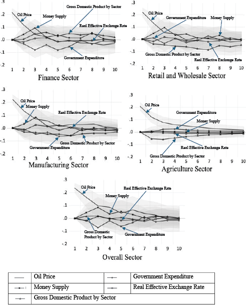
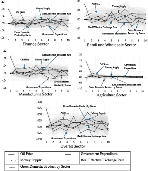
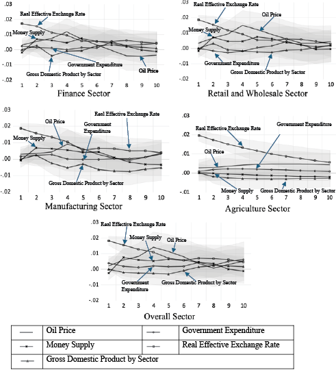
Figure 2 presents the findings from the SVAR impulse response functions, illustrating the responses of the Government expenditure to shocks in the oil price, Government expenditure, money supply, real effective exchange rate, and GDP across various sectors in Malaysia. Oil price shocks consistently triggered positive responses in the Government expenditure across all sectors, thus highlighting the sensitivity of fiscal policies to energy prices. Government expenditure shocks showed varied responses, with mixed effects in the finance, retail, wholesale and manufacturing sectors, while the agriculture sector stabilised after initial positive impacts. Money supply shocks had mainly positive effects, with short-term stabilisation in the retail, wholesale, and agriculture sectors. Real effective exchange rate shocks led to sector-specific responses, with most sectors stabilising early on, followed by positive impacts, particularly in the finance, manufacturing, and retail. GDP shocks showed mixed effects, with stabilisation or positive impacts in the finance and agriculture, and alternating responses in retail, wholesale, and manufacturing.

Figure 3. Impulse Response Function of Money Supply to Shocks in Oil Price, Government Expenditure, Money Supply, Real Effective Exchange Rate or Gross Domestic Product by Finance, Retail and Wholesale, Manufacturing, Agriculture and Overall sectors

Notes: See Figure 1 for explanation.

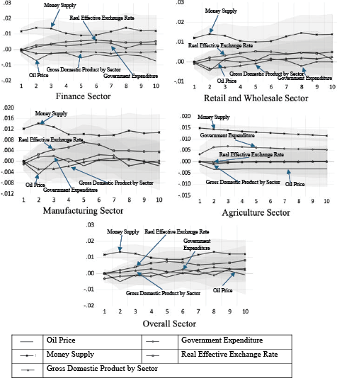
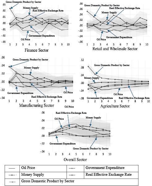
Figure 3 presents the SVAR impulse response functions, showing the dynamic responses of the money supply to shocks in the oil price, Government expenditure, money supply, real effective exchange rate, and GDP across Malaysia’s sectors. In the finance sector, the money supply initially responded negatively to the oil price and GDP shocks, but positively to the Government expenditure, money supply, and real effective exchange rate shocks. The retail and wholesale sector exhibited a transient negative response to the oil price and GDP shocks, while stabilising later, with mixed responses to the Government expenditure and positive impacts from the money supply and real effective exchange rate shocks. The manufacturing sector showed alternating responses to the oil price shocks, positive effects from the money supply and real effective exchange rate, and a negative response to GDP, stabilising near zero. In agriculture, the oil price shocks had a sustained negative impact, while the Government expenditure and money supply triggered positive responses, with the real effective exchange rate effects being neutral. Overall, the sectoral trends showed initial negative impacts from the oil price and Government expenditure shocks, later shifting to positive effects, alongside consistent positive responses to the money supply, real effective exchange rate, and GDP shocks.

Figure 4 presents the SVAR impulse response function, showing how the real effective exchange rate responds to shocks in the oil price, Government expenditure, money supply, real effective exchange rate and GDP across Malaysia’s sectors. The finance sector showed mostly positive responses to the oil price, Government expenditure and exchange rate shocks, but negative responses to the money supply and GDP shocks, thereby indicating mixed sensitivities. The retail and wholesale sector exhibited persistent positive responses to the oil price and exchange rate shocks, with mixed responses to the Government expenditure, money supply and GDP shocks, thus reflecting exposure to both policy and market dynamics. The manufacturing sector responded positively to the oil price, Government expenditure and exchange rate shocks, yet it faced negative impacts from the money supply and GDP shocks, which suggests vulnerability to monetary and sectoral disturbances. The agriculture sector had strong positive responses to the oil price, Government expenditure and exchange rate shocks, but consistently negative responses to the money supply and GDP shocks, thus highlighting external and policy dependence. The overall sector showed stable positive responses to the oil price, Government expenditure and exchange rate shocks, while responses to the money supply and GDP shocks varied, thereby indicating resilience to economic shocks.

Figure 5 presents the SVAR impulse response function results, highlighting the sectoral responses to shocks in the oil price, Government expenditure, money supply and real effective exchange rate across Malaysia’s sectors. The finance sector experienced negative impacts from the oil price and money supply shocks, while GDP responded positively to the real effective exchange rate and its own shocks. The retail and wholesale sector showed persistent negative reactions to the oil price shocks, with mixed responses to policy factors. The manufacturing sector had a stable positive response to the money supply and GDP shocks, but limited sensitivity to exchange rate changes. The agriculture sector faced negative impacts from the oil price, Government expenditure and exchange rate shocks, while demonstrating resilience to monetary conditions. The overall sector showed positive responses to all shocks, which indicates strong economic integration and the capacity to absorb shocks effectively.

Figure 4. Impulse Response Function of Real Effective Exchange Rate to Shocks in Oil Price, Government Expenditure, Money Supply, Real Effective Exchange Rate or Gross Domestic Product by Finance, Retail and Wholesale, Manufacturing, Agriculture and Overall sectors

Notes: See Figure 1 for explanation.

Figure 5. Impulse Response Function of Gross Domestic Product to Shocks in Oil Price, Government Expenditure, Money Supply, Real Effective Exchange Rate or Gross Domestic Product by Finance, Retail and Wholesale, Manufacturing, Agriculture and Overall sectors

Notes: See Figure 1 for explanation.

Conclusion and Policy Recommendations

In conclusion, this study provides a detailed analysis of how key economic variables – specifically, the oil price, Government expenditure, money supply, and exchange rates – affected Malaysia’s finance, retail and wholesale sectors through variance decomposition and impulse response function analyses by using the SVAR model.

The findings from the SVAR variance decomposition show that the influence of macroeconomic variables – namely, the oil price, Government expenditure, money supply, real effective exchange rate and GDP – on each other increased over time, while their own shocks became less significant. This shift reflects the growing interconnectedness of Malaysia’s economy with global forces and sectoral dependencies. The agriculture sector was less sensitive to monetary and exchange rate fluctuations, and domestic monetary shocks had a diminishing impact on GDP. External factors, such as global commodity prices and fiscal policies, became more influential, which highlights the economy’s reliance on broader economic dynamics.

The SVAR impulse response function analysis has revealed sector-specific responses to shocks such as the oil price, Government expenditure, money supply, exchange rate, and GDP. The finance and retail sectors show positive responses to shocks such as the oil price and GDP, stabilising over time. Manufacturing was sensitive to shocks such as monetary conditions, while agriculture exhibited mixed responses, which reflects its reliance on external factors. Overall, the economy of Malaysia demonstrated resilience to shocks, although sectors such as agriculture and retail were vulnerable to policy and market changes.

The results of this study offer policy implications to enhance Malaysia’s economic resilience and foster sustainable growth in alignment with SDG 8 (Decent Work and Economic Growth). Policymakers should adopt flexible monetary policies which would adjust the money supply to stabilize sectors such as finance, retail and wholesale, which are particularly vulnerable to fluctuations in the oil price and M2. Fiscal policies should focus on strengthening the agriculture sector by supporting innovation and climate resilience initiatives. Effective exchange rate management is vital for maintaining export competitiveness in the manufacturing and wholesale sectors, with a managed floating exchange rate and strategic foreign exchange interventions during periods of volatility. Additionally, the Government should establish an oil price stabilization fund and invest in energy diversification to reduce its reliance on oil exports. Promotion of economic diversification, particularly in technology and renewable energy, will further enhance resilience to external shocks. Lastly, fostering cross-sectoral coordination between ministries is essential for creating integrated policy frameworks which would ensure long-term economic stability and growth.

Future research could explore the nonlinear relationships between macroeconomic variables and sectoral dynamics by using advanced methods like Threshold Vector Autoregression (TVAR) or machine learning. Investigation of emerging factors such as environmental sustainability, digital transformation and technological innovation could offer deeper insights into sector-specific trends. Comparative studies with other ASEAN countries could improve the understanding of regional interconnectedness and policy responses. Additionally, examination of the long-term impacts of global economic shocks, such as the climate change or geopolitical tensions, would help develop more adaptive and resilient economic policies.

References

Abdullah, H., El-Rasheed, S., & Khan, H. H. A. (2022). Asymmetric impact of exchange rate changes on money demand in Malaysia. Contemporary Economics, 16(3), 317–328. https://doi.org/10.5709/ce.1897-9254.484

Abubakar, A. B., Muhammad, M., & Mensah, S. (2023). Response of fiscal efforts to oil price dynamics. Resources Policy, 81, 103353. https://doi.org/10.1016/j.resourpol.2023.103353

Al Jabri, S., Raghavan, M., & Vespignani, J. (2022). Oil prices and fiscal policy in an oil-exporter country: Empirical evidence from Oman. Energy Economics, 111, 106103. https://doi.org/10.1016/j.eneco.2022.106103

Blanchard, O. J., & Quah, D. (1989). The dynamic effects of aggregate demand supply disturbances. American Economic Review, 79, 665–673.

Cenc, H. (2022). Government expenditure and economic growth in Euro Area countries. Naše Gospodarstvo/Our Economy, 68(2), 19–27. https://doi.org/10.2478/ngoe-2022-0008

Charfeddine, L., Klein, T., & Walther, T. (2020). Reviewing the oil price–GDP growth relationship: A replication study. Energy Economics, 88, 104786. https://doi.org/10.1016/j.eneco.2020.104786

Coscieme, L., Mortensen, L. F. anderson, S., Ward, J., Donohue, I., & Sutton, P. C. (2020). Going beyond gross domestic product as an indicator to bring coherence to the Sustainable Development Goals. Journal of Cleaner Production, 248,119232. https://doi.org/10.1016/j.jclepro.2019.119232

Crispín, A. R. M., Morales, S. A. G., Rivera, A. S. M., Santos, Á. O. L., & Carrasco, O. A. B. (2023). Structural analysis with SVAR model of the effectiveness of fiscal policy in Peru: 1995–2019. Journal of Law and Sustainable Development, 11(6), e1201. https://doi.org/10.55908/sdgs.v11i6.1201

Dudzevičiūtė, G., Šimelytė, A., & Liučvaitienė, A. (2018). Government expenditure and economic growth in the European Union countries. International Journal of Social Economics, 45(2), 372–386. https://doi.org/10.1108/IJSE-12-2016-0365

Kriskkumar, K., Naseem, N. A. M., & Azman-Saini, W. N. W. (2022). Investigating the asymmetric effect of oil price on the economic growth in Malaysia: Applying augmented ARDL and nonlinear ARDL techniques. Sage Open, 12(1). https://doi.org/10.1177/21582440221079936

Lal, M., Kumar, S., Pandey, D. K., Rai, V. K., & Lim, W. M. (2023). Exchange rate volatility and international trade. Journal of Business Research, 167, 114156. https://doi.org/10.1016/j.jbusres.2023.114156

Leng, J. (2013). The differentiated research of China’s monetary policy’s effect on stock price under the SVAR model—Empirical analysis based on different economic backgrounds. British Journal of Economics, Management & Trade, 3(4), 429–441. https://doi.org/10.9734/BJEMT/2013/4527

Mandler, M., Scharnagl, M., & Volz, U. (2022). Heterogeneity in Euro Area monetary policy transmission: Results from a large multicountry BVAR model. Journal of Money, Credit and Banking, 54(2–3), 627–649. https://doi.org/10.1111/jmcb.12859

Manning, P. (2024). The impact of US housing demand supply shocks on the Australian economy: Analysis implementing a SVAR model. Australian Economic Papers, 63(S1), 79–88. https://doi.org/10.1111/1467-8454.12348

Nach, M., & Ncwadi, R. (2024). Evaluating BRICS as an optimum currency area: Insights from SVAR modelling. Cogent Economics & Finance, 12(1). https://doi.org/10.1080/23322039.2024.2399321

Neusser, K., & Kugler, M. (1998). Manufacturing growth and financial development: Evidence from OECD countries. Review of Economics and Statistics, 80(4), 638–646. https://doi.org/10.1162/003465398557726

Onafowora, O., & Owoye, O. (2019). Impact of external debt shocks on economic growth in Nigeria: A SVAR analysis. Economic Change and Restructuring, 52(2), 157–179. https://doi.org/10.1007/s10644-017-9222-5

Poku, K., Opoku, E., & Agyeiwaa Ennin, P. (2022). The influence of government expenditure on economic growth in Ghana: An ARDL approach. Cogent Economics & Finance, 10(1). https://doi.org/10.1080/23322039.2022.2160036

Raduzzi, R., & Ribba, A. (2020). The macroeconomic outcome of oil shocks in the small Eurozone economies. The World Economy, 43(1), 191–211. https://doi.org/10.1111/twec.12862

Sims, C. A. (1980). Macroeconomics and reality. Econometrica, 48(1), 1. https://doi.org/10.2307/1912017

Sui, J., Lv, W., Gao, X., & Koedijk, K. G. (2024). China’s GDP-at-risk: Real-time monitoring, risk tracing and macroeconomic policy effects. Journal of International Money and Finance, 147, 103150. https://doi.org/10.1016/j.jimonfin.2024.103150

Taghizadeh-Hesary, F., Yoshino, N., Rasoulinezhad, E., & Chang, Y. (2019). Trade linkages and transmission of oil price fluctuations. Energy Policy, 133, 110872. https://doi.org/10.1016/j.enpol.2019.07.008

Tan, C.-T., Mohamed, A., Habibullah, M. S., & Chin, L. (2020). The impacts of monetary and fiscal policies on economic growth in Malaysia, Singapore and Thailand. South Asian Journal of Macroeconomics and Public Finance, 9(1), 114–130. https://doi.org/10.1177/2277978720906066

Trabelsi, R. (2024). Sources of macroeconomic fluctuations in Tunisia: A structural VAR approach. SN Business & Economics, 4(10), 111. https://doi.org/10.1007/s43546-024-00717-3

Van Eyden, R., Difeto, M., Gupta, R., & Wohar, M. E. (2019). Oil price volatility and economic growth: Evidence from advanced economies using more than a century’s data. Applied Energy, 233–234, 612–621. https://doi.org/10.1016/j.apenergy.2018.10.049

Wang, Y., Wang, X., Zhang, Z., Cui, Z., & Zhang, Y. (2023). Role of fiscal and monetary policies for economic recovery in China. Economic Analysis and Policy, 77, 51–63. https://doi.org/10.1016/j.eap.2022.10.011

Yildirim, Z., & Guloglu, H. (2024). Macro-financial transmission of global oil shocks to BRIC countries—International financial (uncertainty) conditions matter. Energy, 306, 132297. https://doi.org/10.1016/j.energy.2024.132297

Zhu, H., Yu, D., Hau, L., Wu, H., & Ye, F. (2022). Time-frequency effect of crude oil and exchange rates on stock markets in BRICS countries: Evidence from wavelet quantile regression analysis. North American Journal of Economics and Finance, 61. https://doi.org/10.1016/j.najef.2022.101708