Ekonomika ISSN 1392-1258 eISSN 2424-6166

2026, vol. 105(4), pp. 24–42 DOI: https://doi.org/10.15388/Ekon.2026.105.4.2

Threshold Effects of Import Dependence on Domestic Output and GVA Multipliers across Ukraine’s Economic Sectors

Lyubomyr Sozanskyy
Department of Problems of the Real Sector of the Economy of Regions,
State Institution “Dolishniy Institute of Regional Research of the NAS of Ukraine”, Ukraine
https://orcid.org/0000-0001-7854-3310
e-mail:ls.ird2@ukr.net

Abstract. This study examines how import dependence, measured as the imported inputs’ share of intermediate consumption, affects the domestic output and gross value added (GVA) multipliers across Ukraine’s economic activities. By using OECD national input–output tables for 1995–2022, two individual dynamic threshold regressions are estimated for each of 49 activities, with activity-specific lags and deterministic trends. A common threshold for both multipliers is identified empirically rather than imposed a priori.
The relationship is nonlinear: below the threshold, higher import dependence raises the multipliers or has no statistically significant effect; above it, both decline. Estimated thresholds range from 6.79% in forestry and logging to 37.47% in coke and refined petroleum products. In 2022, 42 of 49 activities exceeded their thresholds, thus indicating a widespread cross-sectoral pattern.
The analysis establishes three economic regularities. First, the threshold at which imported inputs cease to support domestic production and begin to displace it is common to both multipliers, linking weaker intersectoral production effects to a reduced domestic value added. Second, the wide dispersion of thresholds calls for sector-differentiated rather than aggregate localisation policy. Third, lags of zero to three years reveal differing transmission horizons for changes in import dependence. These findings provide activity-specific guidance for Ukraine’s post-war reconstruction.
Keywords: import dependence; threshold regression; domestic multipliers; input–output analysis.

________

Received: 23/01/2026. Accepted: 09/10/2026
Copyright © 2026 Lyubomyr Sozanskyy. Published by Vilnius University Press
This is an Open Access article distributed under the terms of the Creative Commons Attribution License, which permits unrestricted use, distribution, and reproduction in any medium, provided the original author and source are credited.

1. Introduction

The strength of domestic intersectoral linkages determines how effectively an economy transforms the final demand into cumulative production and value-added effects. In Ukraine, intermediate consumption in many activities relies heavily on imported inputs. Within the input–output framework (Miller & Blair, 2022), a higher import share reduces the domestic technical coefficient matrix, compresses the domestic Leontief inverse, and weakens both the output and GVA multipliers. This relationship is unlikely to be linear. Its direction and magnitude may vary with the level of import dependence, defined here as the share of imported intermediate inputs in the total intermediate consumption.

The empirical literature offers conflicting evidence. One strand emphasises a crowding-out mechanism, in which, imported intermediates substitute for domestic production and weaken backward linkages. Another strand highlights the complementary role of imports at moderate levels, where they fill critical gaps and facilitate the formation of new production linkages. These opposing findings point to a common feature: the effect of import dependence is conditional and likely governed by a threshold.

Three complementary frameworks motivate this view. Structural dependency theory (Hirschman, 1958) holds that excessive reliance on external inputs undermines domestic production systems. Input–output analysis formalises this mechanism through the domestic Leontief inverse. The global value chain perspective explains why imports may initially complement domestic production before becoming substitutive at higher levels of dependence. Together, these approaches imply a nonlinear relationship: imported inputs may be beneficial or neutral below a critical level but detrimental to domestic multipliers above it.

Ukraine offers a particularly informative setting. Its economy is structurally diverse and provides substantial cross-sectoral variation in import dependence. The period of 1995–2022 spans post-transition restructuring, the global financial crisis, geopolitical disruptions, and full-scale war, thereby allowing structural rather than cyclical patterns to be identified. In the context of post-war recovery, identifying the threshold levels at which import dependence becomes detrimental is directly relevant to the design of targeted industrial and localisation policies.

Despite growing interest in the topic, a clear gap remains in the literature. Existing threshold studies rely on aggregate data or focus on outcomes other than multipliers, while studies linking imports to multiplier effects typically assume linear relationships. For Ukraine, three questions remain unanswered. The first issue is whether the qualitative change in the response of the output and GVA multipliers is governed by the same critical level of import dependence. The second point is whether this level varies predictably across sectors. Whereas, the third aspect concerns the time that elapses between changes in import dependence and their effect on the multipliers.

This study aims to determine the effects of different levels of import dependence on the domestic output and GVA multipliers of Ukraine’s economic activities and to identify the sectoral regularities of this relationship. Specifically, the analysis estimates the activity-specific threshold, compares threshold dispersion across sectors, and determines the time required for changes in import dependence to be reflected in each multiplier.

The research hypothesis is that the effect of import dependence on domestic multipliers is nonlinear: below a critical threshold, increases in import dependence strengthen the multipliers or have no statistically significant effect, whereas, above it, they reduce both multipliers.

The contribution is threefold. First, the study estimates a common threshold for the output and GVA equations, reflecting their common basis in the domestic Leontief inverse. Second, it documents how this threshold varies across 49 activities with different technological and production characteristics. Third, it combines threshold positions, output and GVA multipliers, and activity-specific lags in a structural typology designed to support differentiated localisation and reconstruction priorities. The remainder of the paper is organised as follows. Section 2 reviews the literature, Section 3 describes the data and methodology, Section 4 presents the results, Section 5 discusses their implications, and Section 6 concludes the paper.

2. Literature Review

The analytical framework is grounded in input–output methodology, which establishes a direct quantitative relationship between intermediate consumption and multiplier effects (Miller & Blair, 2022; Oosterhaven, 2002). A higher share of imported intermediate inputs reduces the domestic technical coefficient matrix and, through the Leontief multiplier process, lowers the cumulative output and value-added effects generated within the domestic economy. Because the output and GVA multipliers are derived from the same domestic Leontief inverse, they respond to changes in the same underlying matrix structure. Standard linear specifications cannot capture responses whose magnitude and direction vary with the level of import dependence (Kolokontes, 2021).

This nonlinearity helps reconcile conflicting evidence. Above a critical level, imported intermediates may substitute for domestic suppliers and weaken backward linkages. This pattern has been documented across many economies (Ayas, 2017; Backinezos et al., 2020; Basher, 1997; Bui Trinh et al., 2008; Kubo, 1985; Mujeri & Alauddin, 1994; Nealy, 2020; Nguyen, 2021). At moderate levels, however, imports may fill technological or resource gaps and complement domestic production (Amaral et al., 2016; Arriola et al., 2024; Bouattour et al., 2024; Davies, 2006; Kordalska & Olczyk, 2021). The two mechanisms may therefore operate on opposite sides of a threshold.

The location of this threshold and its variation across sectors remain unresolved. Existing threshold analyses aggregate the impact of imports at the GDP level without sectoral disaggregation (Aigheyisi, 2021), or focus on supply security and the geographic concentration of dependencies (Méjean & Rousseaux, 2024; Sultan & Matthes, 2025; Magerman & Consonni, 2025). For Ukraine, Ishchuk and Sozanskyy (2024, 2025) and Ilyash et al. (2021) provide detailed sectoral measures of import dependence by using input–output tables. None of these studies, however, has addressed three questions. The first is whether the level at which the relationship between import dependence and multipliers changes is common to the output and GVA equations. The second question is how this level varies across sectors with different technological content. Whereas, the final question is how much time elapses between changes in import dependence and their effect on the multipliers.

Despite this convergence of theoretical mechanisms and empirical evidence, three questions central to localisation policy remain unresolved within a sectorally disaggregated national framework. The first concerns the level at which the relationship between imported inputs and domestic multipliers changes qualitatively. The second issue is whether the threshold varies systematically across activities with different technological characteristics. Meanwhile, the third aspect concerns the time horizon over which changes in import dependence are reflected in multiplier values. The present study addresses these questions for Ukraine.

The proposed framework, therefore, extends existing studies in two respects. It moves from aggregate measures of import dependence to activity-specific thresholds and examines the output and value-added multipliers jointly rather than as separate outcomes. This joint perspective is important for two reasons. An activity may sustain production volumes while retaining a diminishing share of domestic value added. Moreover, a single aggregate benchmark can conceal large differences in the capacity of sectors to absorb imported inputs.

3. Data and Methodology

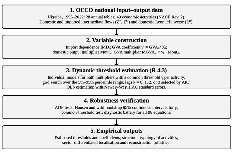
The study proceeds in three stages. First, it constructs the variables for 49 economic activities. Second, it estimates individual dynamic threshold regressions with the objective to identify the import-dependence level at which the multipliers change qualitatively. Third, it verifies robustness and develops a structural typology. Figure 1 summarises the workflow.

Figure 1. Methodological workflow: from OECD source data to verified threshold-regression results.

Source: authors’ own construction.

The analysis uses OECD national input–output tables for Ukraine covering 1995–2022 (OECD, 2025). These tables separate intermediate consumption into domestic (ZD) and imported (ZM) components for 49 NACE Rev. 2 activities. The identical sectoral structure across 28 annual tables yields a balanced dataset of 1,372 observations. Four indicators are constructed from the intermediate-consumption matrices and the domestic Leontief inverse LD. The first is import dependence IMDi. The second is the GVA coefficient vi = GVAi / Xi. The third is the output multiplier Mout,i, defined as the column sum of LD. The fourth is the GVA multiplier MGVA,i = vi · Mout,i. Relative within-year indicators limit the influence of price variation, while long-term dynamics are controlled by a deterministic trend. Import dependence is defined as the share of imported intermediate inputs in total intermediate consumption:

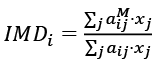(1)

Here, aijM denotes imported input coefficients, aij denotes total technical coefficients, and xj is the sectoral output. An increase in IMDi reduces the domestic coefficient matrix AD and weakens the propagation of domestic production linkages. The dependent variables are Mout,i and MGVA,i.

To capture this nonlinearity, individual dynamic threshold regressions are estimated for each activity (Hansen, 2000; Tang, 2021). Estimation of individual rather than pooled models preserves sectoral differences in production structures, thresholds, and lag patterns. A common threshold γ is estimated for the output and GVA equations because both multipliers are functions of the same domestic Leontief inverse. The models are:

M_out,t = α₁ + β_1,out·IMD_t−k1·I(IMD_t−k1 ≤ γ) + β_2,out·IMD_t−k1·I(IMD_t−k1 > γ) +
θ₁·T + ε_1,t, (2)

M_GVA,t = α₂ + β_1,GVA·IMD_t−k2·I(IMD_t−k2 ≤ γ) + β_2,GVA·IMD_t−k2·I(IMD_t−k2 > γ) +
θ₂·T + ε_2,t, (3)

Here, Mout,t and MGVA,t are the domestic output and GVA multipliers in year t; IMDt−k is import dependence with lag k; and k1 and k2 are the lags for the output and GVA equations. T = {1, …, n} is a deterministic time trend. The indicator I(·) equals one when the stated condition holds; γ is the estimated activity-specific threshold; and ε1,t and ε2,t are the error terms.

The coefficients β1,out and β1,GVA measure the below-threshold responses of the multipliers, while β2,out and β2,GVA measure their responses above the threshold. The intercepts α1 and α2 represent the baseline multiplier levels, and θ1 and θ2 capture average annual changes associated with factors not represented by sectoral import dependence.

The deterministic trend controls for time-related influences not captured by import dependence, while lagged explanatory values reduce the risk of contemporaneous reverse causality.

The empirical design follows the structural logic of the input–output framework. Direct and indirect intersectoral relationships enter the analysis through the construction of both dependent variables from the domestic Leontief inverse. The equations are estimated separately for each activity because cross-sectoral differences in thresholds, coefficients and lags are part of the research question. Pooling would impose restrictions that could conceal this heterogeneity. The 1995–2022 period provides the maximum annual OECD coverage for Ukraine and spans major structural and macroeconomic changes, creating sufficient variation to identify persistent sectoral patterns.

For each activity, γ is identified by grid search between the 5^th and 95^th percentiles of IMDᵢ, by using a one-percentage-point step. The selected value minimises the joint residual sum of squares of the two equations. The lag for each equation is selected from k ∈ {0, 1, 2, 3} by using the Akaike Information Criterion (AIC). Parameters are estimated by OLS with Newey–West HAC standard errors (Newey & West, 1987). In total, 98 models are estimated in R 4.3.

Robustness is assessed through three complementary procedures: sign stability across alternative lags, re-estimation for 1995–2008 and 2009–2022, and Augmented Dickey–Fuller tests of the input series. Appendix A provides a concise summary.

Inference for γ uses Hansen’s (2000) likelihood-ratio-inversion confidence interval and a wild bootstrap with Rademacher multiplier weights and 499 replications per activity (Liu, 1988; Davidson & Flachaire, 2008). A bootstrap likelihood-ratio test evaluates the common-threshold restriction across the output and GVA equations. The results are reported in Section 4.

4. Results

For each of the 49 activities, one threshold regression is estimated for the output multiplier and one for the GVA multiplier, yielding 98 models. All models are statistically significant: adjusted R² values range from 0.701 to 0.899 for the output equations and from 0.701 to 0.896 for the GVA equations. The F-statistics of 18.8–71.2 exceed the critical value at the 1% level. Likelihood-ratio tests confirm the significance of γ for all 49 activities at the 5% level. The post-threshold coefficients are negative and statistically significant under HAC-corrected inference. Appendix A summarises the robustness checks.

The estimates support the research hypothesis by identifying, for every activity, a threshold level of import dependence beyond which both multipliers decline. The threshold is common to the two equations. This is consistent with the fact that the GVA multiplier is a function of the output multiplier and that both depend on the same domestic Leontief inverse. A threshold-related change in that matrix, therefore, affects both multipliers simultaneously.

The estimated thresholds vary substantially, from 6.79% in forestry and logging (A02) to 37.47% in coke and refined petroleum products (C19). Activities for which domestic alternatives are available have lower thresholds. By contrast, sectors dependent on technologically non-substitutable inputs – electricity generation (D35, γ = 36.11%), non-ferrous metallurgy (C24B, 34.54%) and coke manufacturing (C19, 37.47%) – sustain higher dependence before multiplier effects deteriorate. Sectors with stronger GVA generation tend to have lower thresholds, suggesting greater vulnerability in denser domestic value-creation networks.

Figure 2. Sectoral distribution of estimated import-dependence thresholds (γ) across 49 economic activities in Ukraine

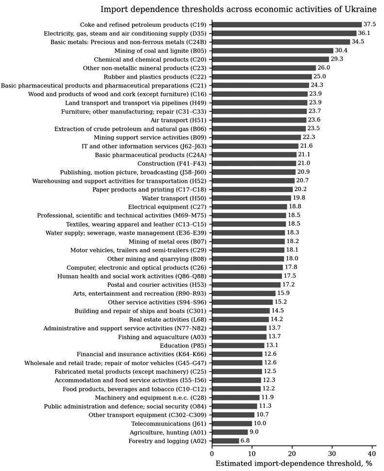
A comparison with the observed import dependence in 2022 shows that 42 out of 49 activities operated above their thresholds. Excessive import dependence is therefore a broad cross-sectoral pattern rather than an outcome confined to individual sectors. Only seven activities remained below γ, in several cases by no more than 0.5 percentage points. The association with multiplier values differs markedly on the two sides of the threshold.

Below γ, an increasing import dependence raises the output multiplier in 25 of 49 activities (β1 > 0, p < 0.05) and the GVA multiplier in 22 activities (β1 > 0). The remaining activities show no significant response. This confirms the complementary role of imports at moderate levels. The strongest output response is observed in other transport equipment (C302–C309): β1 = 4.369, implying an increase of 4.37 cents in domestic output per dollar of final demand for each percentage-point increase in import dependence below γ.

Above γ, the relationship is uniformly negative: both multipliers decline as import dependence increases in all 49 activities. The largest negative output effects are recorded in telecommunications (J61, β2 = −1.645), arts and entertainment (R90–R93, β2 = −1.555), and forestry and logging (A02, β2 = −1.288).

Figure 3 generalises this pattern for the domestic output multiplier by presenting the below- and above-threshold marginal effects and the corresponding value of γ for all activities. The below-threshold effect is positive or near zero in many activities, whereas the above-threshold effect is negative across all activities, with substantial variation in magnitude. Figure 4 illustrates the corresponding output and GVA multiplier profiles for three representative activities.

The estimates also reveal threshold-related asymmetry. Activities that benefit most from import integration below γ tend to experience the largest declines after the threshold is exceeded. The two multipliers can also differ markedly in magnitude. Other transport equipment (C302–C309) illustrates this pattern. Below γ = 10.7%, a one-percentage-point increase in import dependence raises the output multiplier by USD 0.044 per dollar of final demand. Above γ, the output multiplier is virtually insensitive (β2 ≈ 0). The GVA multiplier responds more strongly (β2 = −0.589), declining by approximately USD 0.0059 per unit of final demand for each additional percentage point of import dependence. Thus, physical production may be maintained while the associated domestic value added is lower.

The selected lags range from zero to three years and differ between the output and GVA equations in 39 out of 49 activities. The GVA response appears sooner in 24 activities and later in 15, while the lags coincide in the remaining 10 activities. Short lags are typical of activities with rapid production cycles, whereas capital-intensive industries with complex subcontracting networks have longer adjustment periods. The full effects of localisation policies in such sectors may therefore become visible only after several years.

The deterministic trends reveal an additional pattern: the output multiplier trend is positive in 40 activities and approximately zero in one, while the GVA multiplier trend is negative in 36 activities. Production linkages may therefore expand while the domestic value added they generate contracts. This is consistent with Ukraine’s position in global value chains as a supplier of material-intensive, lower-value-added intermediates and with the pattern of ‘growth without development’ (Yeboah, 2025).

Figure 3. Threshold effects of import dependence for individual sectors on domestic output multipliers across 49 economic activities in Ukraine

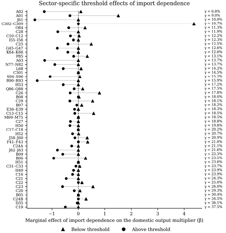
Note: triangle markers denote marginal effects below the threshold (β₁). Circles denote marginal effects above the threshold (β₂). Horizontal segments connect the pre- and post-threshold coefficients for each sector. The symbol γ denotes the estimated import-dependence threshold.

Source: authors’ calculations based on OECD national input–output tables.

Taken together with the lag estimates, this result shows that the weakening of domestic value creation is not necessarily immediate. In activities with longer adjustment periods, changes in imported-input dependence may first alter intermediate sourcing and only later affect the domestic output and GVA generated throughout the production chain. The timing of policy evaluation should therefore reflect the activity-specific lag rather than a uniform annual horizon.

Figure 4. Model-based threshold dependence of domestic output and GVA multipliers on import dependence: A01 Agriculture, hunting; C10–C12 Food products; and C302–C309 Other transport equipment, Ukraine, 1995–2022

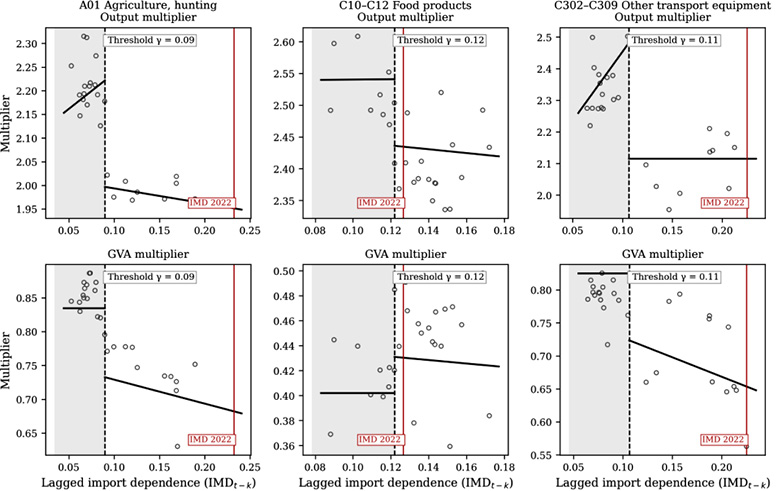
Source: authors’ calculations based on OECD national input–output tables.

To synthesise the findings, activities are classified by using their year 2022 normalised output and GVA multipliers, n_M_out = M_out / 1.918 and n_M_GVA = M_GVA / 0.601, together with their position relative to γ. Values above 1.0 indicate above-average multiplier performance. Table 1 presents the summary characteristics, and Appendix C lists the activities in each type.

Table 1. Structural typology of 49 economic activities by normalised multiplier indices (Ukraine, 2022)

Note: n_M_out and n_M_GVA – normalised output and GVA multipliers; Δγ – average gap from the estimated threshold.

Source: authors’ calculations based on OECD (2025).

Type 1 comprises agriculture (A01), forestry and logging (A02), shipbuilding (C301), and accommodation and food services (I55–I56), for which, both normalised multipliers exceed the economy-wide averages. This type combines the strongest multiplier performance with the lowest average threshold (10.6%). All four activities operated above γ in 2022, with an average gap of 8.0 percentage points. For agriculture and forestry, where β1 > 0, a reduction of dependence towards γ would eliminate the negative post-threshold effect and restore the stimulative below-threshold effect.

Type 2 includes 23 activities forming the industrial core, including machinery and equipment (C28), electronics (C26), chemicals (C20), food products (C10–C12), and basic metals (C24A). Their output multipliers exceed the average, whereas their GVA multipliers are below it. The M_out / M_GVA ratio of 5.71 is the highest of the three types, thus indicating substantial production chains but disproportionately low domestic value-added retention. The GVA multiplier is, therefore, a more informative localisation criterion than the output alone. Coke manufacturing (C19), non-metallic mineral products (C23), non-ferrous metallurgy (C24B), and coal mining (B05) remained below γ in 2022 and are candidates for preventive rather than corrective support.

Type 3 contains 22 activities, including telecommunications (J61), financial services (K64–K66), trade (G45–G47), education (P85), and electricity supply (D35). Their normalised GVA multipliers exceed the average, while their output multipliers are below it. The group is heterogeneous: service activities operate far above γ and show high multiplier sensitivity, whereas electricity supply (D35, γ = 36.11%, β2 = −0.041) displays limited output-multiplier sensitivity despite substantial import dependence. The level of dependence must therefore be assessed together with the magnitude of the multiplier response.

Threshold reliability is assessed by two independent procedures. The average widths of the 95% Hansen and bootstrap confidence intervals are 5.59 and 6.78 percentage points. The corresponding medians are 5 and 7 percentage points. The close agreement between the two procedures supports the stability of γ. The common-threshold restriction H0: γout = γGVA is not rejected for any activity. The median absolute difference between separately estimated thresholds is 4 percentage points (mean 3.71), which is within the mean Hansen interval width. Variance Inflation Factors, Breusch–Pagan and White tests, Durbin–Watson and Breusch–Godfrey tests (Godfrey, 1978), and Engle–Granger residual-stationarity tests using MacKinnon (2010) critical values are applied to the 98 regressions. Newey–West HAC standard errors are used throughout. Appendix A summarises these checks. Appendix B reports the model parameters.

5. Discussion

Taken together, the findings show that the weakening of domestic production linkages and the compression of domestic value added are two manifestations of the same threshold-related change. Because γ varies from 6.79% to 37.47% and transmission lags range from zero to three years, neither a single economy-wide import benchmark nor a uniform policy horizon is appropriate.

First, the negative above-threshold effect in all 49 activities is consistent with the crowding-out mechanism documented by Nguyen (2021), Nealy (2020), Kubo (1985), and Backinezos et al. (2020). The results show, however, that the effect is conditional on γ. Positive below-threshold responses in many activities support the complementary role of imported inputs emphasised by Arriola et al. (2024) and Kordalska and Olczyk (2021). The threshold specification, therefore, reconciles two strands of evidence that appear contradictory under linear models.

Second, the threshold-related asymmetry indicates that activities benefiting most from moderate import integration may suffer the largest losses once γ has been exceeded. This is consistent with structural dependency theory (Hirschman, 1958): dense domestic production networks generate strong multipliers but also create multiple points of vulnerability to import substitution. Differences between the output and GVA responses are also consistent with limited value-added capture in peripheral global value chain positions (Gereffi et al., 2005).

Third, positive output-multiplier trends and negative GVA-multiplier trends in many activities indicate that domestic value-added retention may decline even without additional import dependence. This pattern is consistent with ‘growth without development’ (Yeboah, 2025), and also with evidence on Central and Eastern European functional specialisation (Kordalska & Olczyk, 2021). Reducing import dependence is therefore necessary but not sufficient; it should be accompanied with technological and functional upgrading.

The policy implications differ by structural type. Monitoring each activity’s gap from γ would distinguish sectors requiring active localisation from those needing preventive measures. Type 1 combines high output and GVA effects with low thresholds. Type 2 has strong production linkages but weak domestic GVA retention, making the GVA multiplier the more informative priority criterion. Type 3 requires instruments adapted to service and digital value chains. The lag structure also implies that policy outcomes should be assessed over horizons longer than one budget cycle.

In practical terms, the threshold should be treated as a sector-specific monitoring benchmark rather than a universal import target. Activities already above γ require measures aimed at rebuilding domestic supplier capacity and substituting imported intermediates where technologically feasible. Activities still below γ require preventive monitoring, support for domestic suppliers, and safeguards against rapid increases in dependence. For industrial activities, priorities should be based jointly on the output multiplier, the GVA multiplier, and the size of the above-threshold gap.

The results should be interpreted within the study’s scope. The regressions identify conditional threshold relationships rather than a structural causal mechanism, and the estimated values reflect Ukraine’s production structure. Lagged specifications mitigate but do not eliminate simultaneity. OECD data end in 2022, and therefore do not capture subsequent wartime and reconstruction changes. Future research can strengthen causal identification and test the approach in other Central and Eastern European economies.

Comparative application to Poland, the Czech Republic and other Central and Eastern European economies would help distinguish Ukraine-specific thresholds from regularities associated with transitional production structures. Instrumental-variable approaches could strengthen causal interpretation. Updated post-2022 input–output tables would allow an assessment of how wartime disruption, relocation and reconstruction change the composition of domestic linkages and the location of sectoral thresholds.

6. Conclusions

This study identifies import-dependence thresholds for all 49 economic activities in Ukraine and estimates the nonlinear responses of domestic output and GVA multipliers below and above those thresholds.

The research hypothesis is supported for 1995–2022. Below γ, higher import dependence either raises the multipliers or has no statistically significant effect; above γ, both multipliers decline in all 49 activity models. The result is stable across technological profiles, lag specifications and the macroeconomic episodes covered by the data.

Thresholds reflect differences in the substitutability of imported components and sectoral production technologies. These differences explain why the thresholds range from 6.79% in forestry and logging to 37.47% in coke and refined petroleum products. In 2022, 42 activities operated above their estimated thresholds.

A further contribution is the identified asymmetry: activities with the strongest positive below-threshold responses incur the largest losses after γ has been exceeded. Differences between the output and GVA responses show that physical production can be sustained while domestic value added grows more slowly or declines.

The effects unfold with lags of zero to three years that differ between the two multipliers. The opposing deterministic trends – notably, rising output multipliers and declining GVA multipliers in many activities – also show that a reduction in import dependence must be complemented with structural upgrading within global value chains.

The study, therefore, makes three substantive contributions: it identifies a common threshold for the output and GVA multipliers in each activity; it demonstrates substantial cross-sectoral variation in γ; and establishes the sectoral time horizons over which changes in import dependence affect multiplier dynamics. The resulting typology provides an operational basis for differentiated localisation and reconstruction policy.

For reconstruction policy, the results imply that import substitution should not be applied uniformly. The relevant objective is to move activities with excessive dependence towards their own estimated thresholds while preserving imported inputs that remain complementary to domestic production. Joint use of the output and GVA multipliers helps identify whether stronger production linkages are accompanied with adequate retention of domestic value added.

Future research should compare the thresholds with those of Central and Eastern European economies and apply instrumental-variable approaches to strengthen causal interpretation. The analysis should also be repeated when post-2022 input–output tables become available to assess how wartime disruption and reconstruction reshape production networks, thresholds and multiplier dynamics.

References

Aigheyisi, O. S. (2021). Threshold effects of import dependence on economic growth in Nigeria. ACTA VSFS, 15(2), 198–219. https://acta.vsfs.eu/pdf/acta-2021-2-04.pdf

Amaral, A. E., de Campos, A. C., Sesso Filho, U. A., Esteves, E. G. Z., & Brene, P. R. A. (2016). Linkages of the processing sectors in the Brazilian economy through the internalization of imported intermediate inputs. Proceedings of the 44th ANPEC Meeting. ANPEC. https://www.anpec.org.br/encontro/2016/submissao/files_I/i9-c0a8d22a65e9b752392fda8c32f2ec97.pdf

Arriola, C., Cai, M., Kowalski, P., Miroudot, S., & van Tongeren, F. (2024). Towards demystifying trade dependencies: At what point do trade linkages become a concern? OECD Trade Policy Papers, No. 280. OECD Publishing. https://doi.org/10.1787/2a1a2bb9-en

Ayas, N. (2017). Import dependency of sectors and major determinants: An input–output analysis. European Journal of Sustainable Development Research, 2(1), 1–16. https://doi.org/10.20897/ejosdr.201701

Backinezos, C., Panagiotou, S., & Vourvachaki, E. (2020). Multiplier effects by sector: An input–output analysis of the Greek economy. Economic Bulletin, 52, 7–28. Bank of Greece. https://ideas.repec.org/a/bog/econbl/y2020i52p7-28.html

Basher, M. A. (1997). Linkages and leakages: A sectoral tracking in the Bangladesh economy. The Bangladesh Development Studies, 25(1–2), 71–94. https://ideas.repec.org/a/ris/badest/0370.html

Bouattour, A., Kalai, M., & Helali, K. (2024). Threshold effects of technology import on industrial employment: A panel smooth transition regression approach. Journal of Economic Structures, 13(1), 1–33. https://doi.org/10.1186/s40008-023-00322-x

Breusch, T. S., & Pagan, A. R. (1979). A simple test for heteroscedasticity and random coefficient variation. Econometrica, 47(5), 1287–1294. https://doi.org/10.2307/1911963

Bui Trinh, Pham Le Hoa, & Bui Chau Giang. (2008). Import multiplier in input–output analysis (DEPOCEN Working Paper Series No. 2008/23). Development and Policies Research Center. http://depocenwp.org/upload/pubs/BuiTrinh/Import%20multiplier%20in%20input_DEPOCENWP.pdf

Davidson, R., & Flachaire, E. (2008). The wild bootstrap, tamed at last. Journal of Econometrics, 146(1), 162–169. https://doi.org/10.1016/j.jeconom.2008.08.003

Davies, R. (2006). Manufacturing employment and import dependence. Human Sciences Research Council. https://www.gtac.gov.za/wp-content/uploads/2022/02/Manufacturing-Employment-and-Import-Dependence.pdf

Dickey, D. A., & Fuller, W. A. (1979). Distribution of the estimators for autoregressive time series with a unit root. Journal of the American Statistical Association, 74(366), 427–431. https://doi.org/10.2307/2286348

Engle, R. F., & Granger, C. W. J. (1987). Co-integration and error correction: Representation, estimation, and testing. Econometrica, 55(2), 251–276. https://doi.org/10.2307/1913236

Gereffi, G., Humphrey, J., & Sturgeon, T. (2005). The governance of global value chains. Review of International Political Economy, 12(1), 78–104. https://doi.org/10.1080/09692290500049805

Godfrey, L. G. (1978). Testing against general autoregressive and moving average error models when the regressors include lagged dependent variables. Econometrica, 46(6), 1293–1301. https://doi.org/10.2307/1913829

Hansen, B. E. (2000). Sample splitting and threshold estimation. Econometrica, 68(3), 575–603. https://doi.org/10.1111/1468-0262.00124

Hirschman, A. O. (1958). The strategy of economic development. Yale University Press.

Ilyash, O., Lupak, R., Vasyltsiv, T., Trofymenko, O., & Dzhadan, I. (2021). Modelling of the dependencies of industrial development on marketing efficiency, innovation and technological activity indicators. Ekonomika, 100(1), 94–116. https://doi.org/10.15388/Ekon.2021.1.6

Ishchuk, S., & Sozanskyy, L. (2024). Modelling the impact of manufacturability and import dependence on the efficiency of the processing industry of Ukraine. Studies of the Industrial Geography Commission of the Polish Geographical Society, 38(2), 49–68. https://doi.org/10.24917/20801653.382.3

Ishchuk, S., & Sozanskyy, L. (2025). The impact of economic globalization on the import dependence and product innovativeness of manufacturing industry: A case study of France, Germany, Italy and Poland. Studies of the Industrial Geography Commission of the Polish Geographical Society, 39(4), 7–28. https://doi.org/10.24917/20801653.394.1

Kolokontes, A. D. (2021). Reposition of forward-to-backward input-output analysis. Scientific Annals of Economics and Business, 68(2), 195–232. https://doi.org/10.47743/saeb-2021-0015

Kordalska, A., & Olczyk, M. (2021). New patterns in the position of CEE countries in global value chains: Functional specialisation approach. Oeconomia Copernicana, 12(1), 35–52. https://doi.org/10.24136/oc.2021.002

Kubo, Y. (1985). A cross-country comparison of interindustry linkages and the role of imported intermediate inputs. World Development, 13(12), 1287–1298. https://doi.org/10.1016/0305-750X(85)90126-3

Liu, R. Y. (1988). Bootstrap procedures under some non-i.i.d. models. The Annals of Statistics, 16(4), 1696–1708. https://doi.org/10.1214/aos/1176351062

MacKinnon, J. G. (2010). Critical values for cointegration tests (Working Paper No. 1227). Queen’s Economics Department. https://www.econ.queensu.ca/sites/econ.queensu.ca/files/qed_wp_1227.pdf

Magerman, G., & Consonni, N. (2025). Quantifying EU strategic dependence [ECARES Working Paper]. Université libre de Bruxelles. https://static1.squarespace.com/static/55e85d72e4b0146280523def/t/6883a31a01f3e40ee4f7e1e3/1753457436048/quantifying_strategic_dependence.pdf

Méjean, I., & Rousseaux, P. (2024). Identifying European trade dependencies. In J. Pisani-Ferry, B. Weder di Mauro, & J. Zettelmeyer (Eds.), Paris Report 2: Europe’s Economic Security. CEPR Press. https://cepr.org/publications/books-and-reports/paris-report-2-europes-economic-security

Miller, R. E., & Blair, P. D. (2022). Input–output analysis: Foundations and extensions (3rd ed.). Cambridge University Press. https://doi.org/10.1017/9781108676212

Mujeri, M. K., & Alauddin, M. (1994). Trade and linkages using an input–output approach: An empirical investigation of Bangladesh. The Pakistan Development Review, 33(1), 75–92.

Nealy, M. (2020). Economy changing over time. IMPLAN Support. https://support.implan.com/hc/en-us/articles/360049768074-Economy-Changing-Over-Time

Newey, W. K., & West, K. D. (1987). A simple, positive semi-definite, heteroskedasticity and autocorrelation consistent covariance matrix. Econometrica, 55(3), 703–708. https://doi.org/10.2307/1913610

Nguyen, H. T. (2021). Intersectoral linkages and imports of Vietnam: An input–output approach. International Journal of Economic Policy Studies, 15(1), 205–231. https://doi.org/10.1007/s42495-021-00057-2

OECD. (2025). Input–output tables [Data set]. https://www.oecd.org/en/data/datasets/input-output-tables.html

Oosterhaven, J. (2002). On the dynamics of net versus gross multipliers [Paper presentation]. 42nd Congress of the European Regional Science Association, Dortmund. https://hdl.handle.net/10419/115551

Sultan, S., & Matthes, J. (2025). U.S. dependence on imports from the EU (IW-Report, No. 41). German Economic Institute. https://www.iwkoeln.de/en/studies/samina-sultan-juergen-matthes-us-dependence-on-imports-from-the-eu.html

Tang, C. F. (2021). The threshold effects of educational tourism on economic growth. Current Issues in Tourism, 24(1), 33–48. https://doi.org/10.1080/13683500.2019.1694869

White, H. (1980). A heteroskedasticity-consistent covariance matrix estimator and a direct test for heteroskedasticity. Econometrica, 48(4), 817–838. https://doi.org/10.2307/1912934

Yeboah, E. (2025). The effect of foreign direct investment, domestic investment, and trade on economic growth: Evidence from the Baltic countries. Ekonomika, 103(4), 129–150. https://doi.org/10.15388/Ekon.2024.103.4.8

Appendix A. Robustness Verification

Stationarity was tested for all 49 activities by using the Augmented Dickey–Fuller (ADF) test (Dickey & Fuller, 1979). The import-dependence series IMDᵢ are first-order non-stationary: the unit-root null is not rejected in levels (mean p = 0.42) but is rejected in first differences (mean p < 0.01). The output and GVA multiplier series are trend-stationary, with the unit-root null rejected in levels under a trend specification (mean p < 0.05). The deterministic trends in Equations (2)–(3), therefore, account for the common time component and mitigate the risk of spurious dependence.

Sign stability is confirmed across all specifications: β2,out < 0 and β2,GVA < 0 in all 49 activities and across lags k ∈ {0, 1, 2, 3}, yielding no sign deviations in 392 estimated models. Re-estimation for 1995–2008 and 2009–2022 produces the same signs and closely similar magnitudes, thereby indicating that the results are not driven by one macroeconomic episode.

Illustrative diagnostic report (water supply; sewerage and waste management, E36–E39). The Breusch–Pagan (Breusch & Pagan, 1979) and White (1980) tests do not reject homoskedasticity at the 5% level. The Breusch–Godfrey tests (Godfrey, 1978) of orders 1 and 2 do not reject the absence of serial correlation. Variance Inflation Factors are below 10. The Engle–Granger procedure (Engle & Granger, 1987; MacKinnon, 2010) confirms residual cointegration at the 5% level. Inference uses Newey–West HAC standard errors, which are robust to heteroskedasticity and serial correlation. The post-threshold effect is significant at p < 0.05 at the AIC-selected lag. Complete diagnostic results for all activities are available from the author upon reasonable request.

Appendix B. Full Model-Parameter Tables

Tables B.1 and B.2 report parameters for all 98 models (two equations per activity, 49 activities, Ukraine, 1995–2022). Activities are listed in NACE Rev. 2 order. Threshold values γ are expressed as proportions (e.g., γ = 0.090 = 9.0%).

Table B.1. Parameters of threshold regression equation (2) for the output multiplier (M_out,i), 49 activities, Ukraine

Note: γ – threshold (proportion), identified by minimising RSSout(γ) + RSSGVA(γ) over the 5^th–95^th percentile grid of IMDi (step 0.01). k1 – time lag for Eq. (2), selected from {0, 1, 2, 3} by AIC. α1 – intercept; β1,out – below-threshold slope; β2,out – above-threshold slope; θ1 – trend coefficient; R̄² – adjusted R². Statistical inference is based on Newey–West HAC standard errors. The key post-threshold effects are significant at p < 0.05 across the 49 activities at the AIC-selected lag.

Source: authors’ calculations based on OECD (2025).

Table B.2. Parameters of threshold regression equation (3) for the GVA multiplier (MGVA_,i), 49 activities, Ukraine

Note: γ – threshold (proportion), common to Equations (2) and (3). k2 – time lag for Eq. (3), selected from {0, 1, 2, 3} by AIC. α2 – intercept; β1,GVA – below-threshold slope; β2,GVA – above-threshold slope; θ2 – trend coefficient; R̄² – adjusted R². Statistical inference is based on Newey–West HAC standard errors. The key post-threshold effects are significant at p < 0.05 across the 49 activities at the AIC-selected lag.

Source: authors’ calculations based on OECD (2025).

Appendix C. Full list of economic activities by structural type

Note: n_M_out = M_out,2022 / 1.918; n_M_GVA = M_GVA,2022 / 0.601 (economy-wide averages, 2022).

Source: authors’ calculations based on OECD (2025).