Organizations and Markets in Emerging Economies ISSN 2029-4581 eISSN 2345-0037
2025, vol. 16, no. 1(32), pp. 193–216 DOI: https://doi.org/10.15388/omee.2025.16.8

The Role of the Underground Economy in the Oil Wealth-Growth Nexus: New Insight from Nigeria

Joseph David
Universiti Pendidikan Sultan Idris, Malaysia
josephdavid970@gmail.com
https://ror.org/005bjd415

Awadh Ahmed Mohammed Gamal (corresponding author)
Universiti Pendidikan Sultan Idris, Malaysia
awadh.gamal@fpe.upsi.edu.my
https://ror.org/005bjd415

Sultan Ali Mohammed Salem
Najran University, Saudi Arabia
sultan260403@gmail.com
https://ror.org/05edw4a90

K. Kuperan Viswanathan
Haas School of Business, UC Berkeley,
United States
kuperan@haas.berkeley.edu

Norasibah Abdul Jalil
Universiti Pendidikan Sultan Idris, Malaysia
norasibah@fpe.upsi.edu.my
https://ror.org/005bjd415

Abstract. Research on the relationship between oil wealth and economic growth has shown that the impact of oil can depend on various factors or conditions. However, the role of the underground economy in this relationship remains underexplored. This study aims to fill this gap by examining how the underground economy influences the oil wealth-growth nexus in Nigeria from 1990 to 2022, using the bootstrap autoregressive distributed lag (ARDL) bounds-testing technique. The empirical findings reveal that the effect of oil wealth on economic growth varies with the size of the underground economy. Specifically, the results indicate that the marginal impact of oil wealth on growth is positive when the underground economy is relatively small, but becomes negative as the underground economy expands. This suggests that the underground economy serves as a channel through which oil wealth negatively affects long-term economic growth. The economic implication of this finding is that for sustained long-term growth, increases in oil wealth must be accompanied by significant efforts to reduce the size of the underground economy.

Keywords: oil wealth, underground economy, economic growth, bootstrap ARDL

Received: 8/7/2024. Accepted: 27/1/2025
Copyright © 2025 Joseph David, Awadh Ahmed Mohammed Gamal, Sultan Ali Mohammed Salem, K. Kuperan Viswanathan, Norasibah Abdul Jalil. Published by Vilnius University Press. This is an Open Access article distributed under the terms of the Creative Commons Attribution Licence, which permits unrestricted use, distribution, and reproduction in any medium, provided the original author and source are credited.

1. Introduction

Over the last few decades, scholars have widely regarded natural resources and the wealth associated with them as a ‘curse’ (Sachs & Warner, 1995). This conclusion is primarily influenced by the relatively poor economic performance of nations with abundant natural resources compared to the significant economic growth and development experienced in resource-poor countries such as Taiwan, Singapore, and Hong Kong (David et al., 2024). Both anecdotal and empirical evidence confirm the validity of this phenomenon in several resource-rich countries across Africa, the Middle East, Europe, Latin America, and Asia. In the literature on the resource curse, it is reported that the adverse effects of natural resource wealth on growth may be transmitted through channels such as weak institutions, corruption, terms of trade, investment, openness, and education, among others (David et al., 2025; Eregha & Mesagan, 2020; Papyrakis & Gerlagh, 2004).

However, little is known about the capacity of the underground economy¹ to act as a transmission channel for the negative impact of natural resource wealth on long-term growth in resource-dependent economies. In the case of oil, for instance, it can be argued that the effect of oil wealth (or revenue) on long-term growth may be influenced by the size of the underground economy in oil-rich countries. This argument is hinged on two key issues. First, the expansion of the underground economy directly erodes the tax base, leading to a reduction in tax revenue and forcing governments to seek alternative means of financing their expenditures (Mazhar & Méon, 2017). Second, evidence suggests that higher oil rents tend to diminish the state’s willingness to tax its citizens, delaying necessary tax reforms (Bornhorst et al., 2009; McGuirk, 2013; Ross, 2001). Conversely, a decline in oil rents often increases the government’s willingness to adopt and implement tax reforms to boost revenue (Ishak & Farzanegan, 2020).

In this context, the prevailing size of the underground economy may determine how oil rent fluctuations impact economic growth by influencing the government’s ability to generate higher tax revenues. Ishak and Farzanegan (2020), for instance, found that in oil-rich countries where the underground economy accounts for more than 35 percent of GDP, a decline in oil rents has a limited effect on raising tax revenues. In contrast, countries with a smaller underground economy may experience an increase in tax revenue following changes in oil rents, with minimal adverse effects on economic growth. However, where the underground economy is extensive, economic growth is likely to be hindered, as efforts to increase tax revenue are often unsuccessful.

The negative shocks in global oil prices in 2009, 2015, and 2020 led to significant declines in oil rents and capital outflows in oil-dependent countries, including Nigeria (World Bank, 2024). The resulting drop in revenue raised Nigeria’s fiscal deficit and increased public debt from 27.6 percent of GDP in 2019 to 35 percent in 2021 (Central Bank of Nigeria [CBN], 2022). Despite a series of non-oil tax reforms, the Nigerian government has struggled to achieve higher tax revenues (CBN, 2022; Herbert et al., 2018), while real GDP and per capita income have continued to decline (World Bank, 2024). The situation has been aggravated by the COVID-19 pandemic and oil theft in the oil-rich Niger Delta region, raising concerns about fiscal sustainability and long-term economic growth. Notably, with the underground economy averaging around 56.8 percent of official GDP during the 1991–2017 period (Medina & Schneider, 2019), the size of the underground economy may play a significant role in the relationship between oil revenue fluctuations and economic growth.

Against this backdrop, we aim to assess whether the effect of oil wealth on economic growth is influenced by the size of the underground economy in Nigeria. In the literature, most research has focused either on the relationship between oil wealth and growth (see Asiedu et al., 2021; Dada & Abanikanda, 2019; David et al., 2024; Eregha & Mesagan, 2020; Inuwa et al., 2022; Ofori & Daryn, 2021; Olayungbo & Adediran, 2017) or on the determinants and effects of the underground economy on economic growth (see Ajide & Dada, 2024; Ajide et al., 2024; Dada et al., 2024; Camara, 2022; Gamal et al., 2025; Goel et al., 2018; Nguyen et al., 2022). Although the conclusions on the impact of oil wealth and the underground economy on growth are mixed and remain inconclusive, the existing literature on the resource curse has largely overlooked the underground economy as a transmission channel, despite its significant presence in various economies. Substantial efforts have instead focused on validating the resource curse through other transmission channels, such as the Dutch disease, resource price variability, rent-seeking, human capital, savings-investment, and money-inflation mechanisms (David et al., 2024; Eregha & Mesagan, 2020; Papyrakis & Gerlagh, 2004).

Our analysis adopts an approach similar to that of David (2024), which investigates how the negative effects of oil prices on economic growth in oil-rich economies are transmitted through corruption. Using a quarterly time-series dataset for the period 1990–2022, we apply the bootstrap autoregressive distributed lag (ARDL) bounds testing methodology to demonstrate that the underground economy is a crucial channel through which oil wealth exerts a significant negative impact on long-term growth. The findings reveal that, while oil wealth promotes economic growth, the underground economy undermines long-term growth prospects, with the marginal effect of oil wealth depending on the size of the underground economy. Specifically, the positive impact of oil wealth on growth is stronger when the underground economy is relatively small, whereas an extensive underground economy allows oil wealth to impede growth. We highlight the need for a country to achieve sustained long-term growth by coupling increase in oil wealth with substantial efforts to reduce the size of the underground economy.

In this paper, we make three important contributions. First, we provide a pioneering analysis of how the size of the underground economy influences the impact of oil wealth on economic growth. Focusing on Nigeria—a major oil-producing country characterised by a history of unimpressive economic performance and a large underground economy—offers a unique opportunity to investigate the validity of the resource-curse phenomenon through the lens of the underground economy. Second, by employing the novel bootstrap autoregressive distributed lag (ARDL) model, we address issues such as weak size and power properties and inconclusive inferences in traditional econometric approaches. This technique allows us to draw more accurate conclusions regarding the long-run relationship between oil wealth, the underground economy, and growth. Additionally, the use of high-frequency quarterly data enhances the robustness and precision of our findings. Lastly, the findings of this study are expected to rekindle debate on the topic and extend the frontiers of knowledge among economists, researchers, policy analysts, and policymakers in Nigeria, as well as in other oil-rich countries and beyond.

The paper proceeds as follows. Section 2 presents the stylised facts on oil wealth, the underground economy, and the Nigerian economy. In Section 3, we outline the theoretical framework, specify the model, and describe the data used in the study. This section also discusses the econometric technique employed. Section 4 is dedicated to the results, beginning with an examination of the stationarity properties of the data, followed by the findings from the bounds-testing procedure and the main empirical results. The policy implications of these findings are also discussed in Section 4. Finally, Section 5 concludes the study.

2. Stylised Facts on Oil Wealth, the Underground Economy
and the Nigerian Economy

Nigeria’s economy is significantly shaped by its dependence on oil and the pervasive presence of the underground economy. These two factors, intertwined with the country’s structural economic challenges, have profound implications for its growth and development. As one of the largest oil producers in Africa, oil has long played a dominant role in Nigeria’s economy. Since the discovery, exploitation, and subsequent exportation of crude oil, it has continued to play a critical role in the nation’s fiscal and monetary policy, providing over 90 per cent of foreign exchange earnings and more than 70 percent of public revenue (CBN, 2022; World Bank, 2024). Data from the World Bank indicate that oil has generated over US$942.517 billion for Nigeria’s coffers between 1970 and 2021, with an average of US$25.936 billion accrued annually during the 1990–2021 period (see Figure 1). Despite contributing only 8 to 10 percent to the Gross Domestic Product (GDP), oil’s significance lies in its role as the primary source of fiscal revenue and foreign exchange. While Nigeria’s abundant crude oil reserves have supported the economy through increased revenue, infrastructural development, and foreign investment, the country’s heavy reliance on oil has also made it vulnerable to the volatile nature of global oil prices (David et al., 2024). This dependency has resulted in cyclical periods of economic boom during high prices and recessionary pressures when prices fall.

The effects of oil price fluctuations are evident. For instance, while the oil booms of the early 1970s, 2007/2008, and 2011/2012 boosted the country’s revenue potential and overall economic performance, negative shocks in global oil prices in 2009, 2015, and 2020 led to significant declines in oil revenue and economic contractions. As shown in Figure 1, positive shocks in oil prices in 1996, 2008, 2011, and 2018 led to increases in oil revenue and corresponding economic growth rates of 4.196 percent, 6.764 percent, 5.308 percent, and 1.923 percent, respectively. In contrast, the economy contracted from 5.308 percent in 2008 to 4.23 percent in 2009; from 6.309 percent in 2014 to 2.653 percent in 2015 and -1.617 percent in 2016; and from 2.208 percent in 2019 to -1.794 per cent in 2020 following negative oil price shocks. These downturns also led to a widening fiscal deficit and an increase in public debt, rising from 27.6 per cent of GDP in 2019 to 35 per cent in 2021 (CBN, 2022). Despite the considerable wealth accrued from oil sales, Nigeria continues to struggle with translating oil revenues into sustainable development outcomes, such as poverty reduction, infrastructural improvements, and inclusive economic growth, which reflects the symptoms of the “resource curse.”

Figure 1
Plots of Nigeria’s Economic Growth Performance, Oil Rent and Underground Economy

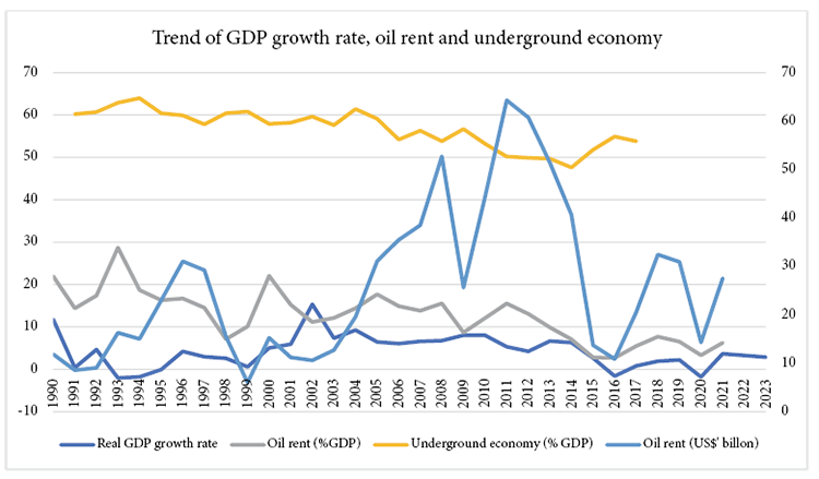
Note. Authors’ computation based on data from World Bank’s World Development Indicators (WDI) and Medina and Schneider (2019).

Simultaneously, Nigeria has one of the largest underground economies in Africa (Dada et al., 2024). According to estimates by Medina and Schneider (2019), the underground economy relative to GDP between 1991 and 2017 ranged from 47.6 percent to 60 percent, with an average of 56.78 percent (see Figure 1). The underground economy encompasses a variety of informal economic activities, including unregistered businesses, informal employment, tax evasion, and illegal trade (Sakanko et al., 2024). Several factors contribute to its substantial size, such as high poverty rates, widespread unemployment, inadequate financial inclusion, and the prevalence of cash-based transactions (Abu et al., 2022c; Dada et al., 2024; Sakanko et al., 2024). The underground economy serves as a vital source of income and employment for a significant portion of the population, particularly in rural areas and among the urban poor (Ajide et al., 2024; Ishak & Farzanegan, 2022). While the underground economy helps alleviate poverty and provide goods and services that may not be available through formal channels, its expansion poses challenges. Evidence shows that it undermines tax revenue collection, complicates macroeconomic management, and impedes the development of formal economic institutions, among other adverse consequences (Medina & Schneider, 2019; Sakanko et al., 2024).

The relationship between oil wealth and the underground economy in Nigeria is complex and often symbiotic. Like most countries with abundant natural resources and heavy reliance on them, high oil revenues have reduced the government’s incentive to broaden the tax base and enhance tax enforcement, allowing the underground economy to flourish. This dependence on oil revenues diminishes the urgency to develop alternative revenue sources, resulting in limited fiscal capacity to invest in public goods and services. As argued by Ishak and Farzanegan (2020), reliance on oil revenues has made efforts to increase public revenue following declines in oil revenue largely ineffective, pushing more individuals into the underground economy. The prevalence of corruption, inefficient bureaucracy, and weak economic institutions further exacerbate the situation. Moreover, economic downturns triggered by falling oil prices push more economic activities into the underground economy. Reduced formal job opportunities and cutbacks in public expenditure during periods of low oil revenue force individuals and businesses to resort to informal economic activities for survival. Ultimately, the country’s dependence on oil has not only made it susceptible to external shocks but has also facilitated the growth of the underground economy by weakening incentives for formal economic development.

3. Theoretical Background, Data, and Methodology

3.1 Theoretical background

A comprehensive theory explaining the role of the underground economy in the oil wealth-growth relationship is challenging to find. However, a link between oil wealth, the underground economy, and economic growth can be forged through the well-known “resource curse” hypothesis (RCH) popularized by Sachs and Warner (1995) and the Ishak-Farzanegan model of the oil rent-taxation-shadow economy relationship (Ishak & Farzanegan, 2020). According to the RCH, countries rich in natural resources, such as oil, often experience slower economic growth compared to resource-poor countries due to factors like economic volatility, institutional weaknesses, and misallocation of resources (Dada & Abanikanda, 2019; David et al., 2024; Sachs & Warner, 1995). The underground economy can exacerbate these challenges by amplifying the negative impacts associated with resource dependence. In resource-rich economies, substantial oil revenues may reduce incentives for governments to diversify the economy or develop strong institutions, leading to weaker regulatory frameworks (Brunnschweiler, 2008; Leite & Weidmann, 1999; Mehlum et al., 2006). This can allow the underground economy to thrive, as businesses and individuals may seek to avoid taxes and regulations that are perceived as burdensome or corrupt (Dada et al., 2024).

The presence of a large underground economy can further undermine the positive impact of oil wealth on economic growth by reducing public revenues, which are crucial for investments in infrastructure, education, and healthcare. Additionally, the underground economy may encourage rent-seeking behavior, corruption, and inefficiencies in resource allocation, all of which contribute to the “resource curse” by distorting economic incentives and reducing the effectiveness of public policies (Eregha & Mesagan, 2020; Dada et al., 2024; David, 2024; David et al., 2024). This position is supported by the Ishak-Farzanegan model, which demonstrates that underground economic activities impede government taxation efforts in oil-dependent economies during economic downturns induced by negative oil price shocks, thereby limiting the government’s ability to finance essential public goods through taxation. In this context, the underground economy acts as an intermediary that intensifies the resource curse, turning oil wealth into a source of economic instability and long-term growth constraints, rather than a driver of development. Thus, the relationship between oil wealth, the underground economy, and economic growth can be conceptualized as a cyclical interaction, where the expansion of the underground economy due to weak institutions and oil dependence exacerbates the negative outcomes predicted by the RCH.

3.2 Model specification

Following some studies (Abu et al., 2022b; David, 2024; David et al., 2025), an econometric model is specified to demonstrate how the oil wealth-growth relationship depends on the size of the underground economy as follows:

yt = α + ψ₁oilt + ψ₂uet + ψ₃ (oilt × uet) + ϑ'Zt + μt (1)

where yt is economic growth (proxy by real GDP), oilt represents oil wealth (measured by the ratio of oil revenue to GDP), uet denotes the underground economy (proxy by the ratio of the share of the underground economy to the official GDP), and Z't is the vector of control variables (such as gross government debt, domestic investment, exchange rate, access to electricity, headline consumer price inflation, and primary fiscal balance). In addition, α, ψ₁ and ψ₂ represent the intercept and the slope coefficients of oil revenue and the underground economy, respectively. ψ₃is the parameter of the interaction term, and ϑ is the vector of the coefficient of control variables. μt denotes the stochastic error terms with zero mean and constant variance. To reduce skewness, real GDP is log transformed before analysis, while the percentage change in the headline consumer price index is computed.

Through the interaction term between oil wealth and the underground economy, the marginal effect of changes in oil wealth on growth can be captured through the partial derivatives of Equation (1) with respect to oil wealth as follows:

(2)

To determine whether the oil wealth-growth relationship is contingent on the size of the underground economy, we focus on the signs of ψ₁ and ψ₃ , as they have fundamental policy implications. First, if ψ₁ and ψ₃ are positive, it implies that oil wealth stimulates economic growth, and an increase in the size of the underground economy intensifies this effect. Second, if the coefficients have different signs, it signals the presence of a threshold effect, implying that the impact of oil wealth on growth varies with the size of the underground economy.

3.3 Data sources and description

This research uses quarterly data covering the 1990–2022 period. Quarterly real GDP and exchange rate (domestic currency (Naira) per the US Dollar, period average) are sourced from the IMF’s International Financial Statistics (IFS) database, while the data for the gross general government debt (% of GDP), primary fiscal balance (the difference between total public revenue and expenditure, excluding net interest payments on public debt, relative to the GDP), and domestic investment (ratio of gross capital formation to the GDP) are extracted from the IMF’s World Economic Outlook (WEO). The quarterly headline consumer price inflation is from the World Bank’s global database of inflation (Ha et al., 2021). In addition, data on infrastructure (percentage of the population with access to electricity) is sourced from the World Bank’s World Development Indicators (WDI) database, while oil revenue (relative to the current GDP) data is from the Central Bank of Nigeria’s (CBN) statistical bulletin. Lastly, the data for the underground economy is from the shadow economy database computed by Medina and Schneider (2019). As the available data for the underground economy do not meet the requirements for time series analysis, the Denton (1971) interpolation procedure is employed to convert the annual data (including the underground economy, gross debt, domestic investment, access to electricity, and oil revenue) into quarterly figures. The robustness and advantages of this procedure are well documented in the literature (see David et al., 2024, 2025).

Table 1
Descriptive Statistics and Correlation Analysis

	y	oil	ue	debt	dinv	fx	elec	fbal	p
Mean	26.371	10.815	55.915	33.739	16.593	146.551	47.767	-1.248	4.154
SD	0.475	5.925	4.638	20.551	4.067	115.795	8.331	4.336	4.443
Min.	25.725	2.323	47.149	7.060	10.331	7.901	24.071	-10.017	-4.667
Max.	27.012	24.075	64.503	75.714	27.633	445.712	64.355	10.406	22.296
oil	-0.589^a	1.000
ue	-0.889^a	0.484^a	1.000
debt	-0.609^a	0.289^a	0.552^a	1.000
dinv	0.629^a	-0.475^a	-0.532^a	-0.229^a	1.000
fx	0.867^a	-0.606^a	-0.745^a	-0.317^a	0.789^a	1.000
elec	0.916^a	-0.522^a	-0.820^a	-0.573^a	0.649^a	0.869^a	1.000
fbal	-0.329^b	0.658^a	0.211^a	-0.151^a	-0.360^a	-0.403^a	-0.291^a	1.000
p	-0.308^a	0.063	0.347^a	0.316^a	-0.283^a	-0.22^b	-0.279^a	-0.081	1.00

Note. (^a) and (^b) denote statistical significance at 1% and 5% levels, respectively. y = log of real GDP; oil = oil revenue relative to GDP; ue = underground economy relative to the official GDP; debt = gross debt of the central government; dinv = ratio of domestic investment to the GDP; fx = exchange rate of Naira per US Dollar; elec = percentage of population with access to electricity; fbal = primary fiscal balance; p = headline consumer price inflation rate.

The summary of the descriptive statistics and correlation analysis of the variables is presented in the upper and lower panels of Table 1, respectively. The results in Table 1 show that the mean value of real GDP (log-transformed) for the period 1990Q1–2022Q4 is 26.371 (US$315.88 billion), with values ranging from 25.725 (US$148.67 billion) to 27.012 (US$538.18 billion). Additionally, the average share of oil revenue relative to GDP during this period is 10.815 percent. The standard deviation indicates a significant variation in government revenue from oil sales, with the value ranging from 2.323 percent to 24.075 percent of GDP. Furthermore, the results reveal that the average size of the underground economy (relative to the official GDP) is substantial, at about 55.95 percent, with the lowest size during the period being 47.149 percent and the highest being 64.503 percent. Regarding the correlation analysis, the results indicate that oil wealth, the underground economy, public debt, fiscal balance, and headline consumer price inflation are negatively correlated with real GDP. In contrast, the correlation between real GDP and domestic investment, exchange rate, and access to electricity is positive and significant. The pairwise correlation between the variables of interest and the control variables is also presented².

3.4 Estimation technique

The bootstrap bounds-testing technique of McNown et al. (2018) is adopted to estimate the relationship specified in Equation (1). The technique, an extension of the ARDL bounds-testing technique of Pesaran et al. (2001), addresses the weak size and power properties associated with the traditional bounds-testing method (McNown et al., 2018). This is achieved by introducing an additional co-integration test on the lagged level(s) of the independent variable(s) to complement the existing F- and t-tests of Pesaran et al. (2001). The introduction of bootstrap-generated critical values also eliminates the problem of inconclusive inferences that characterised the traditional ARDL procedure (David et al., 2024; Gamal et al., 2024).

Generally, a bivariate ARDL(p, q) can be written as follows:

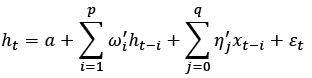(3)

where a, ht and xt represent the constant, response and explanatory variable, respectively. ωi and ηi are the coefficients of the lags of ht and xt , respectively, and εt is the error term. Lastly, i and j are the indexes of lags, i = 1, 2, …, p; j = 0, 1, 2, …, q. t = 1, 2 …, T is time.

We re-parameterise and express Equation (3) in an error correction representation as follows:

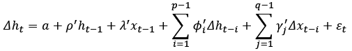(4)

where ∆ is the difference operator. ϕi and γj are functions of ,

and λ = , respectively.

In line with McNown et al. (2018), the co-integration between ht and xt is determined by testing the following hypotheses: H₀ : ρ = λ = 0 (for overall F-test on all lagged-level variables, F₁); H₀ : ρ = 0 (the t-test on the lagged level of the response variable, t); and H₀ : λ = 0 (the F-test on the lagged levels of the explanatory variable(s), F₂). For a valid conclusion on the co-integration between series to be made, all three null hypotheses must be rejected (Abu et al., 2022a; David et al., 2024).

In the case that a co-integrating relationship is established, the long-run estimate is derived by normalising the coefficients of the lagged explanatory variables by the coefficient of lagged dependent variables, that is λ/ρ. A corresponding dynamic short-run error correction model can also be determined as follows.

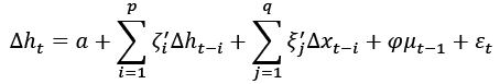(5)

where φ is the parameter of the one-period lag error term (μ_{t – 1}), representing the speed of adjustment back to equilibrium in the long run after a deviation in the short run.

4. Empirical Results and Discussion

4.1 Preliminary data analysis

Before estimating the growth model in Equation (1), the stationarity properties of the variables are assessed using the Augmented Dickey-Fuller (ADF), Phillips-Perron (PP), and Kwiatkowski-Phillips-Schmidt-Shin (KPSS) unit root tests. The unit root test results, summarised in Table 2, present mixed outcomes. Specifically, the ADF and PP test results indicate that all variables, except for headline consumer price inflation, become stationary after first differencing. This suggests that the inflation rate is integrated of order zero (I(0)), while the remaining variables in the model are integrated of order one (I(1)). However, the KPSS test results show that all variables are integrated of order one. Therefore, depending on the test used, the results imply that the variables exhibit a mix of I(0) and I(1) integration orders. Notably, the ARDL bounds-testing procedure remains robust when the variables have a mixed order of integration, as long as they are not integrated of an order higher than one.

Table 2
Results of Unit Root Tests

Test	I(d)	y	oil	ue	debt	dinv	fx	elec	fbal	p
ADF	I(0)	-0.237	-0.620	-0.237	-2.001	-0.834	1.856	-2.471	-1.44	-3.04^**
ADF	I(1)	-2.69^*	-5.31^***	-4.58^***	-3.82^***	-4.62^***	-9.68^***	-4.05^***	-5.81	–
PP	I(0)	-0.49	-1.89	-0.77	-1.99	-1.85	1.82	-2.31	-2.46	-6.63^***
PP	I(1)	-3.35^**	-3.01^**	-2.42	-2.54	-2.77^*	-9.63^***	-2.86^*	-3.04^**	–
KPSS	I(0)	1.39^***	0.76^***	1.22^***	0.67^***	0.79^***	1.26^***	1.42^***	0.47^**	0.39^*
KPSS	I(1)	0.25	0.06	0.08	0.17	0.04	0.09	0.16	0.05	0.07

Note. Asterisks (^***), (^**), and (^*) denote statistical significance at 1%, 5% and 10% levels, respectively. I(d) is the order of integration – I(0) is level and I(1) is first difference. The ADF and PP tests the null of a unit root against the stationary alternative, while the KPSS tests the null of stationarity against unit root alternative. All tests are conducted with intercept (random walk with drift). The optimal lag-length is determined by Schwarz’s (1978) information criteria, while Bartlett kernel and the Newey-West methods are adopted for PP and KPSS tests. MacKinnon’s (1996) critical values (CV) for ADF and PP tests are given as: -3.48 (1%), -2.883 (5%) and -2.579 (10%). KPSS’s CV are: 0.739 (1%), 0.463 (5%), and 0.347 (10%).

4.2 Bootstrap ARDL bounds-testing co-integration

The bootstrap ARDL bounds testing approach is employed to determine the presence or absence of a co-integrating (long-run) relationship between the variables in the specified equation. To ensure robustness, three models are estimated. The first model includes only the variables of interest (oil wealth and the underground economy), the second model replaces the underground economy with the interaction term, and the third model incorporates all the variables of interest (oil revenue, the underground economy) along with their interaction. The results of the bootstrap ARDL bounds testing for the three models are summarised in Table 3. Overall, the results indicate that the values of the three test statistics exceed the bootstrap-generated critical values at the 1% and/or 5% significance levels. Therefore, there is sufficient evidence to reject the null hypothesis of “no co-integrating (long-run) relationship” in all three models.

Table 3
Results of Bootstrap ARDL Bounds-testing

Models	F₁	t	F₂	Bootstrap-generated CVs
Models	F₁	t	F₂	F'₁	F''₁	t'	t''	F'₂	F''₂
Model I	7.375^**	-4.777^**	8.132^**	8.65	7.12	-5.39	-4.55	9.59	7.61
Model II	6.416^***	-4.839^**	6.966^***	5.91	4.80	-4.88	-3.94	6.07	4.95
Model III	26.745^***	-3.887^**	11.242^***	25.70	21.83	-3.57	-2.95	6.16	4.88

Note. Asterisks (^***) and (^**) denote significance at 1% and 5% levels, respectively. Model I is the baseline model of Equation (1) without the oil wealth-underground economy interaction term (Ø't). Model II is the equation with the interaction term (ψ3Ø't), but excluding the underground economy (uet). Model III is Equation (1) – all interest variables and interaction term are included. F₁represents the overall F-statistic for the lagged level variables, F₂ denotes the exogenous F-statistic for the lagged level of the independent variables, and t is the t-statistic for the lagged level of the dependent variable. F'₁, t', and F'₂, andF''₁, t'', and F''₂are the bootstrap generated critical values (with 1,000 replications) at 1% and 5% significance levels, respectively.

4.3 Estimation results of the autoregressive distributed lag model

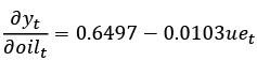
After confirming the presence of a co-integrating relationship between the variables across the three different scenarios, the long-run and short-run models of the selected ARDL model are estimated. The results of the long-run estimates, along with the post-estimation diagnostics, are summarised in Table 4, while the short-run estimates are presented in Table 5. Starting with the assessment of the adequacy and reliability of the estimation results, the post-estimation diagnostics summarised in Panel B of Table 4 indicate that all specifications are free from issues related to serial correlation, heteroscedasticity, and specification bias. Furthermore, the cumulative sum of recursive residuals (CUSUM) and cumulative sum of squares of recursive residuals (CUSUMSQ) plots³ of Brown et al. (1975) confirm the stability of the estimated model parameters. The non-normality of the residuals across all three models, as indicated by the Jarque-Bera statistics, is not coincidental. Evidence suggests that such issues often arise in estimations based on finite sample sizes (David et al., 2024, 2025). As expected, in all three specifications, the error correction term (φμt_–1), which represents the speed of adjustment from short-run disequilibrium to long-run equilibrium, is negative, less than one, and statistically significant at the 1% level. This not only reinforces the presence of co-integration between the series but also indicates the speed at which disequilibrium is corrected: approximately 1.12%, 0.76%, or 2.03% of the short-term disequilibrium is adjusted within a quarter, based on specifications I, II, or III, respectively.

Table 4
Long-run Estimates of Oil, Growth and the Underground Economy Relationship

Regressors	Dependent Δy	Variable:	Model I: ARDL(2,2,4,2,2,2,4,4,2) Model II: ARDL(2,4,4,2,2,0,4,4,2) Model III: ARDL(1,1,1,1,1,0,1,4,2,4)
Regressors	I	II		III
Panel A: Long-run estimates
oil	0.0704 (0.018)^***	0.6497 (0.186)^***		0.0846 (0.026)^***
ue	-0.1062 (0.019)^***			-0.0661 (0.018)^***
oil × ue		-0.0103 (0.003)^***		-0.0066 (0.004)^*
debt	-0.0137 (0.003)^***	-0.0067 (0.004)^*		-0.0131 (0.004)^***
dinv	0.0331 (0.018)^*	0.0539 (0.032)^*		-0.0039 (0.015)
fx	0.0019 (0.001)^**	0.0021 (0.001)^*		0.0052 (0.002)^***
elec	-0.0152 (0.012)	0.0002 (0.015)		-0.0358 (0.017)^**
fbal	-0.0231 (0.013)^*	0.0048 (0.021)		-0.0191 (0.015)
p	0.0498 (0.016)^***	0.0589 (0.027)^**		-0.0295 (0.014)^***
Constant	31.7419 (1.161)^***	24.5179 (0.961)^***		31.1586 (1.386)^***
Panel B: Diagnostics
φμt _{– 1}	-0.0112 (0.001)^***	-0.0076 (0.001)^***		-0.0203 (0.001)^***
χ²SC	4.357 [0.113]	3.675 [0.159]		4.182 [0.124]
χ²FF	0.003 [0.959]	2.338 [0.129]		0.171 [0.679]
χ²JB	6.411 [0.041]	8.269 [0.016]		15.926 [0.001]
Ajd. R²	0.887	0.932		0.604
CUSUM	Stable	Stable		Stable
CUSUMSQ	Stable	Stable		Stable

Note. The specification in Column (I) excludes the interaction term. Column (II) is the specification without the underground economy. For CUSUM and CUSUMSQ, “Stable” imply that the CUSUM and CUSUMSQ statistics are within the 5 percent critical line. All the variables are included in the specification of Column (III). Asterisks (^***), (^**) and (^*) denote statistical significance at 1%, 5% and 10% levels, respectively. Values in (.) are standard error. Values in square parentheses [.] in panel B are the probability values of the LM test statistics. φμt _{– 1}is the coefficient of the error term lagged by a period, indicting the speed of adjustment to long-run equilibrium. χ²SC , χ²JB , and χ²FF denote Breusch-Godfrey’s serial correlation LM test, Jarque-Bera normality test and Ramsey RESET F-statistic, respectively. The model is estimated by setting the maximum lag to 4, while the optimal lag-length is suggested by AIC.

Focusing on the long-run estimates in the second column of Table 4, the results show that oil revenue has a significant long-term impact on economic growth, while the relationship between the underground economy and economic growth is negative and significant at the 1% level. The corresponding short-run estimates in panel A of Table 5 reveal that the immediate effects of oil revenue and the underground economy on economic growth are positive and statistically significant. However, the coefficients of lagged oil revenue and the underground economy are negative.

While the immediate and long-term impacts of rising oil revenue are positive, the negative effect of oil revenue on growth in previous periods can be attributed to the volatility of the commodity, which accounts for over 70% of public revenue. This finding is crucial, as a series of negative shocks to oil revenue in recent years has constrained public finances, increased fiscal deficits and debt, and raised concerns about the country’s fiscal sustainability and long-term growth prospects. The short-term positive impact of the underground economy on growth may be linked to its role in creating jobs, alleviating poverty, reducing income inequality, and serving as an informal safety net during economic volatility, thereby reducing social pressure on the state and stimulating the economy (Ajide & Dada, 2024; Ajide et al., 2024; Dada et al., 2024; Ishak & Farzanegan, 2022; Sakanko et al., 2024). However, its negative long-term impact on growth may be explained by the “destructive cycle” it initiates, including reduced tax revenue, inefficiencies in public policies, and distortions in resource allocation, which significantly outweigh any perceived short-term benefits (Sakanko et al., 2024). These findings are consistent with other studies (see Abubakar & Akadiri, 2022; Dada & Abanikanda, 2019; David et al., 2024; Inuwa et al., 2022) that document a significant positive long-term and short-term impact of oil revenue on output in Nigeria, as well as evidence of a long-term negative effect and short-term positive effect of the underground economy on growth (see Goel et al., 2018; Nguyen & Duong, 2021; Nguyen & Luong, 2020; Younas et al., 2022).

In Column II of Table 4, where only oil revenue and the interaction term are included in the specification, the results show that the long-term impact of oil revenue on economic growth is significant and positive, while the interaction term enters the model with a significant negative coefficient. In contrast, the short-run estimates in Table 5 indicate that oil revenue has an immediate negative effect on economic growth, whereas the coefficient of the interaction term is positive and statistically significant. The results suggest that an increase in oil revenue leads to a short-term decline in economic growth by 0.011 percentage points. However, in the long run, economic growth responds positively to the increase in oil revenue, expanding by 0.649 percentage points. The negative coefficient of the interaction term implies that a simultaneous increase in both oil revenue and the underground economy would result in a deceleration of economic performance by 0.01 percentage points.

The third model includes oil revenue, the underground economy, and their interaction term in the specification. The long-run results in Table 4 indicate that the coefficient of oil revenue is positive and significant at the 1% level, while the underground economy and the interaction term have negative and significant coefficients. Conversely, the short-run results in Panel C of Table 5 show that the coefficients for oil revenue, the underground economy, and their interaction are all positive. Including both oil revenue and the underground economy along with their interaction in the specification reduces the magnitude of the coefficients for both the long- and short-run estimates and weakens the statistical significance of the short-run estimates. In the short run, only the interaction term remains significant, at the 10% level.

Given that the signs of the estimated coefficients (for oil revenue and the interaction term) differ, it is imperative to determine the marginal effect within the sample using the estimated long-run coefficients in Column II as follows:

The marginal effects of oil revenue (relative to GDP) on economic growth, computed at the mean (55.915), minimum (47.149), and maximum (64.503) levels of the underground economy (as a percentage of GDP), are 0.0761, 0.1666, and -0.0120, respectively. This implies that a unit increase in oil revenue would spur economic growth by approximately 0.0761% and 0.1666% at the average and minimum levels of the underground economy, respectively. However, at the maximum level of the underground economy, a unit increase would lead to a deceleration in economic growth by approximately 0.0120 percentage points. Therefore, it is indicative that an increase in oil revenue, coupled with a reduction in the size of the underground economy, is imperative for sustained long-term economic growth. The simultaneous increase in both oil revenue and the size of the underground economy is likely to result in economic slowdown.

Table 5
Short-run Estimates of Oil, Growth and the Underground Economy Relationship

Regressors	Dependent Variable: Δy
		Lag order
	0	1	2	3
Panel A: Model I – ARDL(2,2,4,2,2,2,4,4,2)
Δy		0.9612 (0.028)^**
Δoil	0.0033 (0.001)^***	-0.0030 (0.001)^***	-0.0004 (0.001)	0.0005 (0.001)
Δ(oil × ue)	0.0046 (0.001)^***	-0.0055 (0.001)^***
Δdebt	-0.0016 (0.0003)^***	0.0014 (0.001)^***	-0.0002 (0.001)	-0.0001 (0.0003)
Δdinv	0.0065 (0.001)^***	-0.0053 (0.001)^***
Δfx	0.0001 (0.00003)^**	0.0001 (0.00003)^**	0.0001 (0.00003)^**
Δfbal	0.0021 (0.0003)^***	-0.0021 (0.0003)^***
Δp	0.000002 (0.0001)
Panel B: Model II – ARDL(2,4,4,2,2,0,4,4,2)
Δy		0.8325 (0.0218)^***
Δoil	-0.0105 (0.004)^***	0.0069 (0.007)	0.0045 (0.006)	-0.0117 (0.004)^***
Δ(oil × ue)	0.0003 (0.0001)^***	-0.0002 (0.0001)	-0.0001 (0.0001)	0.0002 (0.0001)^***
Δdebt	-0.0015 (0.0002)^***	0.0009 (0.0002)^***
Δdinv	0.0088 (0.001)^***	-0.0065 (0.001)^***
Δfx	0.0001 (0.00002)^***	0.0001 (0.00002)^***	0.00008 (0.00002)^***	0.00004 (0.00002)^*
Δfbal	0.0021 (0.0003)^***	-0.0022 (0.0003)^***
Δp	-0.0002 (0.0001)^**	-0.0005 (0.0001)^***	-0.0005 (0.0001)^***	-0.0002 (0.0001)^**
Panel C: Model III – ARDL(1,1,1,1,1,0,1,4,2,4)
Δoil	0.0012 (0.002)	-0.0006 (0.003)	0.0009 (0.002)	-0.0038 (0.001)^***
Δue	0.0017 (0.002)	0.0004 (0.002)
Δ(oil × ue)	0.0004 (0.0003)^*	0.00001 (0.0004)	0.0001 (0.0004)	0.0004 (0.0003)^*
Δdebt	-0.0012 (0.0002)^***
Δdinv	0.0027 (0.001)^**
Δelec	0.0005 (0.001)
Δfbal	0.0022 (0.001)^***
Δp	-0.0003 (0.0002)^**

Note. Δ represents first difference operator. The interaction term is excluded in the Model I specification in Panel A. Panel B specification excludes the underground economy variable. All the variables are included in Model III specification presented in Panel III. Asterisks (^***), (^**) and (^*) denote significance at 1%, 5% and 10% levels, respectively. Values in parentheses (.) are the standard error. The models are estimated by setting the maximum lag to 4, while the optimal lag-length is suggested by AIC.

Regarding the control variables in all three specifications, the long-run results indicate that public debt, fiscal balance, access to electricity, and the inflation rate are negatively related to long-term growth. In contrast, the long-term impacts of domestic investment and exchange rates on growth are positive and significant. Interestingly, these outcomes are consistent with existing studies (see David, 2024; David et al., 2024; Ehigiamusoe et al., 2019; Ehigiamusoe & Lean, 2020; Eregha & Mesagan, 2020; Olayungbo & Adediran, 2017).

4.4 Oil, growth and the underground economy: policy implications

The findings from this study are quite revealing and carry important policy implications, which can be summarised as follows. First, regardless of the specification, oil revenue has a significant positive long-run impact on economic growth. This corroborates several existing studies (see Abubakar & Akadiri, 2022; Dada & Abanikanda, 2019; Inuwa et al., 2022; Olayungbo & Adediran, 2017; Rotimi et al., 2021). Thus, the policy implication of these findings is that governments in oil-rich countries should implement policies and reforms aimed at increasing revenue from oil sales. Such actions may include instituting reforms in the oil and gas sector, removing bureaucratic bottlenecks, adopting new technologies in oil extraction, upgrading oil infrastructure, and eliminating corrupt practices in the industry. However, caution should be exercised to avoid a situation where all attention and resources are channelled into the oil and gas sector to the detriment of other sectors of the economy, as this could have far-reaching consequences. Moreover, given the volatile nature of oil prices, the establishment of a sovereign wealth fund (SWF) by the government to mobilise “excess” wealth from oil may provide the state with an opportunity to maintain a stable growth path, independent of fluctuations in oil prices.

Second, we show that the underground economy has a positive long-term impact on economic growth, while its short-term effect is negative. This finding aligns with the results of several studies (see Goel et al., 2018; Nguyen & Duong, 2021; Nguyen et al., 2022; Saunoris, 2018; Schneider & Hametner, 2014; Younas et al., 2022) that demonstrate how the underground economy can stimulate growth in the short term but stifle long-term growth. The short-term positive impact may be attributed to the underground economy’s capacity to create jobs, alleviate poverty, reduce income inequality, and serve as an insurance policy against economic volatility, thereby reducing social pressure on the state and stimulating the economy (Ajide et al., 2024; Ishak & Farzanegan, 2022; Sakanko et al., 2024). However, its negative long-term impact on growth can be explained by the “destructive cycle” it initiates, which includes reduced tax revenue, inefficiencies in public policy, and distortions in resource allocation—factors that negatively affect the overall economy. Moreover, the expansion of the shadow economy may impair long-term growth by providing a safe haven for activities associated with the criminal economy, such as money laundering, kidnapping for ransom, and tax evasion (Aljassmi et al., 2024), all of which threaten economic stability. Thus, any short-term benefits the underground economy may offer are eventually outweighed by its substantial adverse effects in the long term (Sakanko et al., 2024). Given the feedback causality link between the size of the underground economy and the growth of the formal sector (Bilan et al., 2020), it can be argued that significant improvements in formal economic activities could help reverse the negative impact by encouraging firms and individuals to transition to the formal sector, thereby reducing the size of the underground economy. Therefore, the policy implication is that governments and policymakers should take proactive measures to shrink the underground economy by addressing its root causes, such as poverty, unemployment, and weak institutions. According to Sakanko et al. (2024), the size of the underground economy in developing countries could be halved through enhanced access to quality financial products and services, increased opportunities for participation in formal and international trade, economic stability in terms of inflation rates, and the development of the agricultural sector.

Lastly, and most importantly, the study reveals that the size of the underground economy adversely moderates the impact of oil revenue on economic growth in Nigeria. Consequently, the marginal effect of oil revenue varies with the size of the underground economy, with oil wealth having a larger stimulating impact on economic growth when the size of the underground economy is very low, while stifling growth at higher levels of the underground economy. Among other things, this finding is significant to the growing literature on the resource curse hypothesis. Beyond confirming the existence of a resource curse issue, it demonstrates the dependence of the impact of oil revenue on the size of the underground economy. This is evidenced by the diminishing positive impact of oil revenue on long-term growth as the size of the underground economy increases. This provides another perspective on the explanation of the resource curse hypothesis, indicating that the underground economy is an important channel through which the resource curse is transmitted into an oil-rich economy.

Overall, the policy implication of this finding is that reducing the size of the underground economy is fundamental for oil wealth to support long-term economic growth in oil-rich countries such as Nigeria. In other words, an increase in oil wealth coupled with a decrease in the size of the underground economy appears to offer more benefits for long-term economic growth compared to the simultaneous increase in both oil revenue and the size of the underground economy. Besides its deleterious effect on long-term growth, the underground economy also stifles growth through an economy’s dependence on oil. Therefore, the government must intensify and strengthen its efforts to reduce the size of the underground economy to mitigate its impact on the overall economy and oil wealth. To achieve long-term economic benefits from abundant oil resources, countries must implement appropriate monetary and fiscal policies to control the development of the underground economy.

5. Conclusion

The empirical literature on the oil-growth relationship demonstrates that the impact of oil wealth may be dependent on some factors and conditions such as the quality of institutions (including the control of corruption), human capital development, industrialisation, rent-seeking, and economic policies, amongst others. However, little or no attention has been paid to exploring the role of the size of the underground economy in determining how the wealth from oil impacts growth. Therefore, this study seeks to investigate the role of the underground economy in the oil wealth-growth relationship using the bootstrap ARDL bounds testing co-integration method. Evidence from the results demonstrates that oil wealth promotes long-term economic growth, while the long-term impact of the underground economy on growth is negative. In addition, and most importantly, the findings indicate that the marginal effect of oil wealth on economic growth varies with the size of the underground economy. This suggests that the positive impact of oil wealth on economic growth is larger when the size of the underground economy is very low. The economic implication of this finding is that the underground economy is a transmission channel through which the ‘resource-curse’ adverse impact of oil wealth is exerted on economic growth. Therefore, for a long-term economic growth, an increase in oil wealth must be accompanied by a significant reduction in the size of the underground economy. Hence, governments and policymakers must adopt appropriate macroeconomic strategies to reduce the size of the underground economy to enable the country and economy to reap the benefits of oil wealth.

Despite this study’s pioneering effort to examine the role of the underground economy in the relationship between oil rent and economic growth, it is not without limitations. The primary limitation lies in the measurement of the underground economy. The data used, sourced from Medina and Schneider (2019), is based on the multiple indicators multiple cause (MIMIC) approach and is restricted to the 1991–2017 period. Additionally, the analysis is limited to Nigeria, which may affect the generalisability of the findings. However, these limitations do not diminish the policy relevance and unique contributions of this study. Future research could build on this work by incorporating more comprehensive and granular datasets with alternative measures of the underground economy across multiple oil-rich economies and extending the time frame. Such studies could provide deeper insights into how the size of the underground economy influences the impact of oil rent on economic growth.

References

Abu, N., David, J., Gamal, A. A. M., & Obi, B. (2022). Non-linear effect of government debt on public expenditure in Nigeria: Insight from bootstrap ARDL procedure. Organizations and Markets in Emerging Economies, 13(1), 163–182. https://doi.org/10.15388/omee.2022.13.75

Abu, N., David, J., Sakanko, M. A., & Amaechi, B. O. O. (2022). Oil price and public expenditure relationship in Nigeria: Does the level of corruption matter. Economic Studies (Ikonomicheski Izsledvania), 31(3), 59–80.

Abu, N., Sakanko, M. A., David, J., Gamal, A. A. M., & Obi, B. (2022). Does financial inclusion reduce poverty in Niger State? Evidence from logistic regression technique. Organizations and Markets in Emerging Economies, 13(2), 443–466. https://doi.org/10.15388/omee.2022.13.88

Abubakar, I. S., & Akadiri, S. S. (2022). Revisiting oil-rent-output growth nexus in Nigeria: Evidence from dynamic autoregressive lag model and kernel-based regularised approach. Environmental Science and Pollution Research, 29(30), 45461–45473. https://doi.org/10.1007/s11356-022-19034-z

Adebayo, T. S., Udemba, E. N., Ahmed, Z., & Kirikkaleli, D. (221). Determinants of consumption-based carbon emissions in Chile: An application of non-linear ARDL. Environmental Science and Pollution Research, 28, 43908–43922. https://doi.org/10.1007/s11356-021-13830-9

Ahmed, Z., Cary, M., & Le, H. P. (2021). Accounting asymmetries in the long-run nexus between globalization and environmental sustainability in the United States: An aggregated and disaggregated investigation. Environmental Impact Assessment Review, 86. https://doi.org/10.1016/j.eiar.2020.106511

Ajide, F. M., Dada, J. T., Al-Faryan, M. A. S., & Tabash, M. I. (2024). Shadow economy-income inequality nexus: A panel analysis of West African countries. Journal of Economic Policy Reform, 1–23. https://doi.org/10.1080/17487870.2024.2392571

Ajide, F. M., & Dada, J. T. (2024). Globalization and shadow economy: A panel analysis for Africa. Review of Economics and Political Science, 9(2), 166–189. https://doi.org/10.1108/REPS-10-2022-0075

Aljassmi, M., Gamal, A. A. M., Abdul Jalil, N., David, J. & Viswanathan, K. K. (2024). Estimating the magnitude of money laundering in the United Arab Emirates (UAE): Evidence from the currency demand approach (CDA). Journal of Money Laundering Control, 27(2), 332–347. https://doi.org/10.1108/JMLC-02-2023-0043

Asiedu, M., Yeboah, E. N., & Boakye, D. O. (2021). Natural resources and the economic growth of west Africa economies. Applied Economics and Finance, 8(2), 20–32. https://doi.org/10.11114/aef.v8i2.5157

Bilan, Y., Tiutiunyk, I., Lyeonov, S., & Vasylieva, T. (2020). Shadow economy and economic development: A panel cointegration and causality analysis. International Journal of Economic Policy in Emerging Economies, 13(2), 173–193.

Bornhorst, F., Gupta, S., & Thornton, J. (2009). Natural resource endowments and the domestic revenue effort. European Journal of Political Economy, 25(4), 439–446. https://doi.org/10.1016/j.ejpoleco.2009.01.003

Brown, R. L., Durbin, J., & Evans, J. M. (1975). Techniques for testing the constancy of regression relationships over time. Journal of the Royal Statistical Society Series B: Statistical Methodology, 37(2), 149–163.

Brunnschweiler, C. N. (2008). Cursing the blessings? Natural resource abundance, institutions, and economic growth. World Development, 36(3), 399–419.

Camara, M. (2022). The impact of the shadow economy on economic growth and CO2 emissions: Evidence from ECOWAS countries. Environmental Science and Pollution Research, 29, 65739–65754. https://doi.org/10.1007/s11356-022-20360-5

Central Bank of Nigeria. (2022). Central Bank of Nigeria Statistical Bulletin, 33, Central Bank of Nigeria (CBN), Abuja, Nigeria, available at: https://statistics.cbn.gov.ng/cbn-onlinestats/DataBrowser.aspx

Cholette, P. (1984). Adjusting sub-annual series to yearly benchmarks. Survey Methodology, 10, 35–49.

Dada, J. T., & Abanikanda, E. O. (2019). How important is oil revenue in Nigerian growth process? Evidence from a threshold regression. International Journal of Sustainable Economy, 11(4), 364–377.

Dada, J. T., Ajide, F. M., Arnaut, M., & Al-Faryan, M. A. S. (2024). On the contributing factors to shadow economy in Africa: Do natural resources, ethnicity and religious diversity make any difference? Resources Policy, 88, 104478. https://doi.org/10.1016/j.resourpol.2023.104478

David, J. (2024). The role of corruption in the oil price-growth relationship: Insights from oil-rich economies. Economic Change and Restructuring, 57(246). https://doi.org/10.1007/s10644-024-09808-5

David, J., Abu, N., & Owolabi, A. (2025). The moderating role of corruption in the oil price-economic growth relationship in an oil-dependent economy: Evidence from Bootstrap ARDL with a Fourier Function. Alternative Economics, 31(1), 5–30. https://doi.org/10.37075/EA.2025.1.01

David, J., Gamal, A. A. M., Mohd Noor, M. A., & Zakariya, Z. (2024). Oil rent, corruption and economic growth relationship in Nigeria: Evidence from various estimation techniques. Journal of Money Laundering Control, 27(5), 962-979. https://doi.org/10.1108/JMLC-10-2023–0160

Denton, F. T. (1971). Adjustment of monthly or quarterly series to annual totals: An approach based on quadratic minimization. Journal of the American Statistical Association, 66(333), 99–102. https://doi.org/10.1080/01621459.1971.10482227

Ehigiamusoe, K. U., & Lean, H. H. (2020). The role of deficit and debt in financing growth in West Africa. Journal of Policy Modeling, 42(1), 216–234. https://doi.org/10.1016/j.jpolmod.2019.08.001

Ehigiamusoe, K. U., Lean, H. H., & Lee, C. C. (2019). Moderating effect of inflation on the finance–growth nexus: Insights from West African countries. Empirical Economics, 57, 399–422. https://doi.org/10.1007/s00181-018-1442-7.

Eregha, P. B., & Mesagan, E. P. (2020). Oil resources, deficit financing and per capita GDP growth in selected oil-rich African nations: A dynamic heterogeneous panel approach. Resources Policy, 66, 101615. https://doi.org/10.1016/j.resourpol.2020.101615

Gamal, A. A. M., David, J., Noor, M. A. M., Hussin, M. Y. M., & Viswanathan, K. K. (2024). Asymmetric effect of shadow economy on environmental pollution in Egypt: Evidence from bootstrap NARDL technique. International Journal of Energy Economics and Policy, 14(3), 206–215.

Gamal, A. A. M., Salem, S. A. M., David, J., & Gan, P. T. (2025). Investigating the effect of the shadow economy on Malaysia’s economic growth: Insight from a nonlinear perspective. Asian Economic and Financial Review, 15(2), 182–195. https://doi.org/10.55493/5002.v15i2.5290

Goel, R. K., Saunoris, J. W., & Schneider, F. (2018). Growth in the shadows: Effect of the shadow economy on U.S. economic growth over more than a century. Contemporary Economic Policy, 37(1), 50–67. https://doi.org/10.1111/coep.12288

Ha, J., Kose, M. A., & Ohnsorge F. (2021). One-stop source: A global database of inflation. Policy Research Working Paper, 9737. World Bank, Washington, DC.

Herbert, W. E., Nwarogu, I. A., & Nwabueze, C. C. (2018). Tax reforms and Nigeria’s economic stability. International Journal of Applied Economics, Finance and Accounting, 3(2), 74–87. https://doi.org/10.33094/8.2017.2018.32.74.87

Inuwa, N., Adamu, S., Sani, M. B., & Modibbo, H. U. (2022). Natural resource and economic growth nexus in Nigeria: A disaggregated approach. Letters in Spatial and Resource Sciences, 15(1), 17–37. https://doi.org/10.1007/s12076-021-00291-4

Ishak, P. W., & Farzanegan, M. R. (2022). Oil price shocks, protest, and the shadow economy: Is there a mitigation effect? Economics & Politics, 34(2), 298–321.

Ishak, P. W., & Farzanegan, M. R. (2020). The impact of declining oil rents on tax revenues: Does the shadow economy matter? Energy Economics, 92, 104925. https://doi.org/10.1016/j.eneco.2020.104925

Leite, C., & Weidmann, J. (1999). Does mother nature corrupt? Natural resources, corruption, and economic growth. IMF Working Paper (99/85). https://doi.org/10.5089/9781451850734.001

Mazhar, U., & Méon, P. G. (2017). Taxing the unobservable: the impact of the shadow economy on inflation and taxation. World Development, 90, 89–103. https://doi.org/ 10.1016/j.worlddev.2016.08.019

McGuirk, E. F. (2013). The illusory leader: natural resources, taxation and accountability. Public Choice, 154 (3–4). 285-313, doi:10.1007/s11127-011-9820-0

McNown, R., Sam, C. Y., & Goh, S. K. (2017). Bootstrapping the autoregressive distributed lag test for cointegration. Applied Economics, 50(13), 1509–1521. https://doi.org/10.1080/00036846.2017.1366643

Mehlum, H., Moene, K., & Torvik, R. (2006). Institutions and the resource curse. The Economic Journal, 116(508), 1–20. https://doi.org/10.1111/j.1468-0297.2006.01045.x

Nguyen, D. V., & Duong, M. T. H. (2021). Shadow economy, corruption and economic growth: An analysis of BRICS countries. The Journal of Asian Finance, Economics and Business, 8(4), 665–672. https://doi.org/10.13106/jafeb.2021.vol8.no4.0665

Nguyen, M. L. T., Bui, T. N., Thai, T. D., Nguyen, T. T., & Nguyen, H. T. (2022). Shadow economy, corruption, and economic growth: A Bayesian analysis. In International Econometric Conference of Vietnam, Springer International Publishing, Cham, (pp. 747–762). https://doi.org/10.1007/978-3-030-98689-6_49

Nguyen, T. A. N., & Luong, T. T. H. (2020). Corruption, shadow economy and economic growth: Evidence from emerging and developing Asian economies. Montenegrin Journal of Economics, 16(4), 85–94. https://doi.org/10.14254/1800-5845/2020.16-4.7

Ofori, P. E., & Grechyna, D. (2021). Remittances, natural resource rent and economic growth in Sub-Saharan Africa. Cogent Economics and Finance, 9(1), 1979305. https://doi.org/10.1080/ 23322039.2021.1979305.

Olayungbo, D. O., & Adediran, K.A. (2017). Effects of oil revenue and institutional quality on economic growth with an ARDL approach”, Energy and Policy Research, 4(1), 44–54. https://doi.org/10.1080/23815639.2017.1307146

Papyrakis, E., & Gerlagh, R. (2004). The Resource Curse Hypothesis and Its Transmission Channels. Journal of Comparative Economics, 32(1), 181–193. https://doi.org/10.1016/j.jce.2003.11.002

Pesaran, M. H., Shin, Y., & Smith, R. J. (2001). Bounds testing approaches to the analysis of level relationships. Journal of Applied Econometrics, 16(3), 289–326. https://doi.org/10.1002/jae.616

Ross, M. L. (2001). Does oil hinder democracy? World Politics, 53(3), 325–361. https://doi.org/10.1353/wp.2001.0011

Rotimi, M. E., IseOlorunkanmi, O. J., Rotimi, G. G., & Doorsamy, M. (2021). Re-examining corruption and economic growth in oil dependent economy: Nigeria’s case. Journal of Money Laundering Control, 25(3), 526–539. https://doi.org/10.1108/JMLC-06-2021-0057

Sachs, J. D., & Warner, A. M. (1995). Natural resource abundance and economic growth. NBER Working Paper (5398). https://doi.org/10.3386/w5398

Sakanko, M. A., David, J., Abu, N., & Gamal, A. A.M. (2024). Financial inclusion and underground economy nexus in West Africa: Evidence from dynamic heterogeneous panel techniques. Economic Change and Restructuring, 57(8). https://doi.org/10.1007/s10644-024-09589-x

Saunoris, J. W. (2017). Is the shadow economy a bane or boon for economic growth? Review of Development Economics, 22(1), 115–132. https://doi.org/10.1111/rode.12332

Schneider, F., & Hametner, B. (2014). The shadow economy in Colombia: Size and effects on economic growth. Peace Economics, Peace Science and Public Policy, 20(2), 293–325. https://doi.org/10.1515/peps-2013-0059

World Bank (2024). World Development Indicators (WDI). World Bank, Washington, DC, available at: https://datacatalog.worldbank.org/world-development-indicators

Younas, Z. I., Qureshi, A., & Al-Faryan, M. A. S. (2022). Financial inclusion, the shadow economy and economic growth in developing economies. Structural Change and Economic Dynamics, 62, 613–621. https://doi.org/10.1016/j.strueco.2022.03.011

Appendix

Table A1
VIF for Contemporaneous and Lagged Independent Variables

Lags	oil	ue	oil × ue	debt	dinv	fx	elec	fbal	p
Model I
0	0.000	0.000		0.000	0.000	0.000	0.000	0.000	0.000
1	0.000	0.000		0.000	0.000	0.000	0.000	0.000	0.000
2	0.000	0.000		0.000	0.000	0.000	0.000	0.000	0.000
3		0.000				0.000			0.000
4		0.000				0.000			0.000
Model II
0	0.000	0.000	0.000	0.000	0.000	0.000	0.000	0.000	0.000
1	0.000	0.000	0.000	0.000	0.000	0.000		0.000	0.000
2	0.000	0.000	0.000	0.000	0.000	0.000		0.000	0.000
3	0.000	0.000	0.000			0.000			0.000
4	0.000	0.000	0.000			0.000			0.000
Model III
0	0.000	0.000	0.000	0.000	0.000	0.000	0.000	0.000	0.000
1	0.000	0.000	0.000	0.000	0.000	0.000	0.000	0.000	0.000
2	0.000	0.000	0.000
3	0.000		0.000
4	0.000		0.000

Figure A1
Model I CUSUM and CUSUMSQ Plots

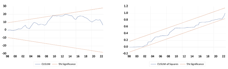
Figure A2
Model II CUSUM and CUSUMSQ Plots

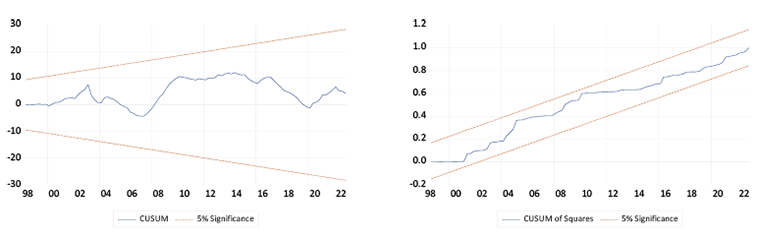
Figure A3
Model III CUSUM and CUSUMSQ Plots

¹In the present study, the underground economy (also referred to as the shadow economy) encompasses all undeclared, under-declared, non-measured, and under-registered production and transactions—both illegal activities associated with crime and corruption, and legal but non-market activities—that intentionally avoid all forms of taxes, minimum wage requirements, safety standards, social security contributions, maximum working hours, administrative procedures, and legal labour market standards (Sakanko et al., 2024).

²We appreciate the anonymous reviewer for highlighting that the strong correlation between the variables of interest and the control variables may raise concerns about multicollinearity. However, it has been noted that the ARDL model can potentially mitigate multicollinearity, as it involves differencing the data to achieve stationarity, which may reduce correlations between the variables (Adebayo et al., 2021; Ahmed et al., 2021). To further investigate this, the variance inflation factor (VIF) was computed for both contemporaneous and lagged independent variables. The results (summarised in Appendix Table A1) show an average VIF of 0.00008, indicating the absence of multicollinearity in the models. Additionally, it is worth noting that one common indicator of multicollinearity is a high R² value combined with insignificant t-statistics for many explanatory variables. However, this pattern is not observed in the results presented in Tables 4 and 5.

³The six CUSUM and CUSUMSQ plots for the three estimated models are presented in the Appendix (Figures A1, A2 and A3).